Beyond OFAT: How Design of Experiments Optimizes Biosensor Development for Biomedical Research
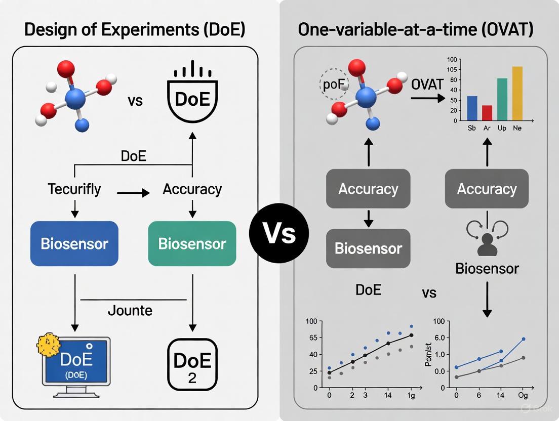
This article explores the critical methodological shift from One-Factor-at-a-Time (OFAT) experimentation to Design of Experiments (DoE) in biosensor development.
Beyond OFAT: How Design of Experiments Optimizes Biosensor Development for Biomedical Research
Abstract
This article explores the critical methodological shift from One-Factor-at-a-Time (OFAT) experimentation to Design of Experiments (DoE) in biosensor development. Aimed at researchers and drug development professionals, it provides a comprehensive analysis of how DoE's multivariate approach efficiently uncovers factor interactions, optimizes complex sensor parameters, and enhances performance metrics like sensitivity and specificity. Drawing on current literature and case studies, the content covers foundational principles, practical applications in electrochemical and optical biosensors, troubleshooting strategies, and a direct comparison of outcomes, offering a actionable framework for developing more reliable and robust sensing platforms for clinical and diagnostic use.
Foundations of Experimental Design: OFAT Limitations and the DoE Paradigm Shift in Biosensing
The development of high-performance biosensors is a complex endeavor, crucial for advancements in personalized healthcare, environmental monitoring, and food safety [1]. The analytical performance of these platforms—their sensitivity, selectivity, and reproducibility—is profoundly affected by the optimization of numerous experimental parameters [2]. Traditionally, this optimization has been dominated by the One-Factor-at-a-Time (OFAT) approach. However, this method is increasingly being supplanted by the statistically rigorous framework of Design of Experiments (DoE) [3] [4]. The choice between these two methodologies is not merely a technical preference but a strategic decision that influences the efficiency, cost, and ultimate success of biosensor development. This guide delineates the core principles of OFAT and DoE, providing researchers and drug development professionals with a clear understanding of their applications, limitations, and strengths within the context of modern biosensor research.
Unpacking the Core Principles
One-Factor-at-a-Time (OFAT): A Sequential Approach
The OFAT approach, also known as One-Variable-at-a-Time (OVAT), is a straightforward, sequential optimization strategy. It involves varying a single experimental factor while keeping all other parameters constant to observe its isolated effect on the response. Once the optimal level for that factor is identified, it is fixed, and the process repeats for the next factor.
- Underlying Logic: The process is based on the assumption that factors are independent and do not interact. The optimal condition for the system is believed to be the simple combination of the individual optimal levels found for each factor.
- Common Contexts: OFAT is widely used in preliminary studies or in systems presumed to be simple. It is often the default method in fields where statistical design is not routinely applied [2] [5].
Design of Experiments (DoE): A Multivariate Paradigm
DoE is a structured, statistical methodology for simultaneously investigating the effects of multiple factors and their interactions on one or more response variables. It is a model-based approach that strategically plans a set of experiments to efficiently explore the entire experimental domain [3].
- Underlying Logic: DoE recognizes that factors in complex systems like biosensors often interact. The effect of one factor (e.g., probe concentration) may depend on the level of another (e.g., ionic strength). DoE aims to build a mathematical model that describes this complex relationship, enabling the identification of a true optimum [2] [5].
- Common Contexts: DoE is the cornerstone of the Quality by Design (QbD) framework mandated by regulatory authorities for pharmaceutical development [4]. It is indispensable for optimizing complex processes with many variables, such as bioprocesses, sensor fabrication, and assay conditions [6] [4].
A Comparative Analysis: OFAT vs. DoE
The fundamental differences between OFAT and DoE lead to significant practical consequences in research outcomes. The table below provides a structured, quantitative comparison.
Table 1: A systematic comparison of OFAT and DoE core characteristics and outcomes.
| Aspect | One-Factor-at-a-Time (OFAT) | Design of Experiments (DoE) |
|---|---|---|
| Experimental Strategy | Sequential, univariate | Simultaneous, multivariate |
| Factor Interactions | Cannot be detected or quantified | Systematically measured and modeled |
| Number of Experiments | Increases linearly with factors; can be very high for complex systems [2] | Increases strategically; highly efficient for many factors [2] |
| Statistical Efficiency | Low; information gained per experiment is limited [7] | High; maximum information for a given number of runs [7] |
| Risk of Sub-Optimality | High; risks missing the true optimum due to ignored interactions [6] [5] | Low; maps the entire response surface to find a robust optimum [6] [5] |
| Foundational Assumption | Factor independence | Factor interdependence (interactions) |
| Model Output | No predictive model | A mathematical model for prediction and optimization |
| Example Efficiency | 486 runs for 6 factors [2] | 30 runs for the same 6 factors (D-optimal design) [2] |
The Critical Concept of Factor Interactions
Factor interactions are a primary reason for DoE's superiority in complex systems. An interaction occurs when the effect of one factor on the response depends on the level of another factor.
For instance, in optimizing a growth medium, the ideal concentration of a carbon source might be different at high and low nitrogen levels. OFAT would completely miss this nuance, while DoE would not only detect it but also quantify it [8]. In biosensor development, interactions are common between parameters like probe concentration, hybridization temperature, and ionic strength [2]. Ignoring them can lead to a sensor with significantly compromised performance.
Experimental Protocols and Case Studies in Biosensor Optimization
Case Study: DoE for a Paper-Based Electrochemical miRNA Biosensor
A compelling example of DoE application is the optimization of a hybridization-based paper-based electrochemical biosensor for detecting miRNA-29c, a biomarker for triple-negative breast cancer [2].
- Objective: Optimize six key variables related to sensor manufacture (e.g., gold nanoparticles, DNA probe concentration) and working conditions (e.g., ionic strength, hybridization time) to improve sensitivity and repeatability.
- Challenge: A full OFAT approach for six variables was estimated to require 486 experiments, which is prohibitively time-consuming and resource-intensive [2].
- DoE Solution: A D-optimal design was selected, which is a computer-generated design that maximizes the information obtained from a limited number of experimental runs.
- Protocol Summary:
- Factor Selection: Six critical factors were identified.
- Experimental Design: A D-optimal design was generated, requiring only 30 experiments.
- Execution & Analysis: The 30 experiments were conducted, and the results (e.g., electrochemical signal intensity) were used to build a statistical model.
- Optimization: The model identified the optimal combination of factor levels and revealed significant interactions between them.
- Outcome: The DoE-optimized biosensor achieved a 5-fold improvement in the limit of detection (LOD) compared to a version optimized using an OFAT strategy. This dramatic enhancement was achieved using 94% fewer experiments [2].
Essential Research Reagent Solutions for Biosensor Optimization
The following table details key materials and reagents commonly used in biosensor optimization experiments, as exemplified in the cited literature.
Table 2: Key research reagents and their functions in biosensor development and optimization.
| Reagent / Material | Function in Biosensor Optimization | Example Context |
|---|---|---|
| Gold Nanoparticles (AuNPs) | Enhance electron transfer, increase surface area for bioreceptor immobilization. | Electrochemical biosensor base modification [2]. |
| Immobilized DNA Probe | Biorecognition element that hybridizes with the target analyte (e.g., miRNA). | miRNA biosensor; concentration is a critical optimized factor [2]. |
| Specific Antibodies | Biorecognition element for immunoassays; binds to target antigen. | Immunosensor for human epididymis protein 4 (HE4) [2]. |
| Nafion | Cation-exchange polymer membrane; improves selectivity and anti-fouling properties. | Modifying electrode surfaces in electrochemical sensors. |
| Magnetic Beads | Solid support for immobilizing bioreceptors; enable separation and concentration of analyte. | Functionalization of antibodies in a competition assay [2]. |
Implementing DoE: A Practical Workflow for Biosensor Development
Adopting a DoE methodology involves a series of logical steps. The following workflow diagram and elaboration provide a guide for its implementation in biosensor research.
- Define Objective and Responses: Clearly state the goal (e.g., "minimize the limit of detection for glucose") and identify the measurable responses that define performance (e.g., current density, signal-to-noise ratio) [2] [1].
- Identify Potential Factors: Brainstorm all possible factors (e.g., pH, temperature, nanomaterial concentration, probe density, incubation time) that could influence the responses [3].
- Screening Design: When dealing with many factors (e.g., >5), use a screening design like a Plackett-Burman or a fractional factorial design to efficiently identify the "vital few" factors that have the most significant impact on the response. This allows for the elimination of insignificant factors, saving resources for the next step [6] [4].
- Optimization Design: Focus on the critical factors identified in the previous step. Use a design like Central Composite Design (CCD), Box-Behnken Design (BBD), or D-optimal design to model the response surface. These designs are capable of estimating quadratic terms and interactions, enabling the location of a true optimum, whether it is a maximum, minimum, or a plateau [2] [3].
- Model Validation and Verification: The final, crucial step is to run a small number of additional experiments at the predicted optimal conditions to verify that the observed response matches the model's prediction. This confirms the model's robustness and validity [3].
The transition from OFAT to DoE represents a paradigm shift from a linear, assumption-heavy approach to a holistic, knowledge-driven one. While OFAT offers simplicity, its inability to account for factor interactions poses a severe risk in the development of complex, high-performance biosensors, often leading to suboptimal performance and a waste of resources [2] [5]. In contrast, DoE provides a systematic, efficient, and statistically sound framework for navigating complex experimental landscapes. It not only finds better optimal conditions but also generates a deeper understanding of the system through the quantification of factor effects and their interactions. As the demand for more sensitive, reliable, and rapidly developed biosensors grows, the adoption of DoE, particularly within the QbD framework, is no longer a luxury but a necessity for researchers and drug development professionals aiming to deliver robust and impactful diagnostic technologies.
In the field of biosensor research, the pursuit of optimal performance—whether in sensitivity, dynamic range, or specificity—often requires careful optimization of multiple experimental parameters. The One-Factor-at-a-Time (OFAT) approach, where variables are altered sequentially while others remain constant, has been a traditional method for this optimization. However, its fundamental inability to capture interactions between factors presents a critical pitfall, often leading researchers to suboptimal outcomes and misleading conclusions. This article details this limitation and contrasts OFAT with the more robust Design of Experiments (DoE) methodology, providing technical guidance and protocols for its implementation within biosensor development.
The Fundamental Flaw: What OFAT Misses
In complex biological systems, such as a functioning biosensor, factors rarely act in isolation. The interaction between two variables occurs when the effect of one factor depends on the level of another. OFAT methodology is inherently incapable of detecting these interactions because it only tests variables individually.
- The Trap of Local Maxima: OFAT involves altering one variable while keeping the others constant, finding its optimal level, and then moving to the next variable. The final combination of variable set points after an OFAT approach is often suboptimal because the outcome is highly dependent on the order in which variables were perturbed. This sequential process can easily trap researchers in a local performance maximum, missing the global optimum that a multivariate approach could find [6].
- Misleading Conclusions: In an OFAT protocol, the impact of a factor is assessed while all other parameters are held constant. This can lead to incorrect conclusions if the optimal level of one factor (e.g., enzyme concentration) shifts when another factor (e.g., buffer pH) is changed. Without testing the full factorial space, these dynamic relationships remain invisible [9].
Table 1: Comparison of OFAT and DoE Approaches in Biosensor Development
| Feature | One-Factor-at-a-Time (OFAT) | Design of Experiments (DoE) |
|---|---|---|
| Factor Interactions | Cannot be detected, leading to suboptimal conditions | Explicitly measured and modeled |
| Experimental Efficiency | Low; requires many runs to explore few factors | High; screens or optimizes many factors with fewer runs |
| Statistical Power | Low; no estimate of experimental error for the full system | High; includes replication for robust error estimation |
| Nature of Solution | Often finds a local optimum | Aims to find the global optimum |
| Best Use Case | Preliminary, rough tuning of a single, dominant factor | Systematic optimization and robust model building |
Case Studies: The Cost of OFAT in Biosensor Research
Optimizing an Electrochemical Biosensor for Metal Ions
In developing a Pt/PPD/GOx amperometric biosensor for detecting heavy metal ions like Bi³⁺ and Al³⁺, researchers turned to DoE to overcome OFAT limitations. The performance was known to be influenced by multiple parameters: enzyme concentration, electropolymerization cycles, and flow rate [10].
An OFAT approach would have optimized one parameter at a time, for instance, finding the best enzyme concentration while keeping cycles and flow rate constant. However, a Central Composite Design (CCD) within a Response Surface Methodology (RSM) framework revealed how these factors interact. The analysis showed that the sensitivity (S, µA·mM⁻¹) was not a simple sum of individual effects but a product of their complex interactions. This allowed the team to identify a true optimal condition (50 U·mL⁻¹ enzyme, 30 cycles, 0.3 mL·min⁻¹ flow rate) that an OFAT search would likely have missed, ultimately achieving high reproducibility (RSD = 0.72%) [10].
Enhancing an RNA Integrity Biosensor
The optimization of an in vitro RNA biosensor highlights the inefficiency of OFAT. With eight different factors to optimize—including reporter protein concentration, poly-dT oligonucleotide concentration, and DTT concentration—an OFAT screen would have been prohibitively time-consuming and resource-intensive [11].
Instead, researchers employed a Definitive Screening Design (DSD), a type of fractional factorial design that efficiently screens many factors with a minimal number of experimental runs. The DSD could model not only the main effects of each factor but also two-factor interactions. This systematic exploration led to an optimized protocol that resulted in a 4.1-fold increase in dynamic range and reduced the required RNA concentration by one-third. The study concluded that key modifications, such as reducing reporter protein and poly-dT concentrations, would have been difficult to identify without a multivariate approach that captured these interactive effects [11].
A Practical Guide to DoE Methodologies for Biosensors
Transitioning from OFAT to DoE involves understanding a suite of statistical tools. The following workflow and descriptions outline the core methodologies.
Core DoE Designs
Screening Designs: These are used when many factors (e.g., pH, temperature, concentration of multiple reagents, buffer ionic strength) are potentially relevant, and the goal is to identify the few most influential ones.
- Plackett-Burman Designs: A highly efficient fractional factorial design used to screen a large number of factors (N) with only N+1 experimental runs. It identifies the main effects of factors but cannot reliably distinguish interaction effects [6].
- Definitive Screening Designs (DSD): A more advanced three-level screening design. DSDs can identify main effects and also model two-factor interactions without a dramatic increase in experimental runs, making them powerful for initial biosensor characterization [11].
Optimization Designs: Once the critical factors are identified, these designs map the response surface to find the optimum.
- Central Composite Design (CCD): A widely used response surface methodology design. It builds upon a two-level factorial design by adding axial (star) points and center points, allowing for the estimation of curvature and quadratic effects. This enables the model to find a maximum or minimum within the experimental region, which is crucial for finding a biosensor's peak performance [10] [9].
- Box-Behnken Design (BBD): Another efficient RSM design. Unlike CCD, Box-Behnken designs do not include points at the extremes (corners) of the factor space, which can be advantageous when testing at these extreme combinations is impractical or impossible [9] [6].
Table 2: Key DoE Designs for Biosensor Development
| DoE Design | Primary Goal | Key Strength | Typical Use in Biosensor Cycle |
|---|---|---|---|
| Full Factorial | Characterize all main effects and interactions | Provides complete data on all factor interactions | Studying a very small number (2-4) of critically important factors in depth |
| Plackett-Burman | Screen a large number of factors to find critical ones | High efficiency; minimal runs for many factors | Initial factor scoping after initial biosensor design |
| Definitive Screening (DSD) | Screen factors while being able to model interactions | Three-level design that captures curvature and interactions | A more robust alternative to Plackett-Burman for screening |
| Central Composite (CCD) | Model curvature and find an optimum | Excellent for building a strong predictive response model | Final performance optimization of critical parameters |
| Box-Behnken (BBD) | Model curvature and find an optimum | Avoids extreme factor combinations; often requires fewer runs than CCD | Optimization when extreme factor levels are undesirable |
Implementing a DoE strategy requires both physical reagents and software tools.
Table 3: Research Reagent Solutions for Biosensor Optimization
| Reagent / Material | Function in Biosensor Optimization |
|---|---|
| Glucose Oxidase (GOx) | Model enzyme used in electrochemical biosensor development; its inhibition by heavy metals is a common detection mechanism [10]. |
| Polymerization Monomers (e.g., o-Phenylenediamine) | Used to form selective polymer membranes on electrode surfaces via electrosynthesis, entrapping enzymes and controlling sensor selectivity [10]. |
| Streptavidin-Coated Magnetic Beads | Solid-phase support for immobilizing biotinylated capture probes (e.g., poly-dT oligonucleotides) in heterogeneous assay biosensors [11]. |
| Dithiothreitol (DTT) | Reducing agent that maintains a stable chemical environment, crucial for the functionality of protein-based biosensor components [11]. |
| Cap Analogs (e.g., ARCA) | Used in in vitro transcription to produce capped mRNA, a key target analyte for RNA integrity biosensors evaluating vaccine quality [11]. |
Software and Statistical Tools:
- Minitab, Design-Expert, JMP: Commercial software packages that provide comprehensive platforms for generating experimental designs, performing ANOVA, and visualizing response surfaces [10] [9].
- DoE Models for Bioreactors App (IDBS Polar): An example of integrated software that automatically calculates statistics and determines significant process parameters from experimental data, a functionality directly transferable to biosensor data analysis [12].
For researchers and drug development professionals working on the cutting edge of biosensor technology, clinging to the OFAT paradigm is a strategic liability. Its critical pitfall—the blindness to factor interactions—compromises performance, undermines reproducibility, and wastes precious resources. The adoption of DoE is no longer a niche advanced practice but a necessary component of rigorous, efficient, and successful biosensor research and development. By embracing the multivariate frameworks outlined in this guide, scientists can systematically navigate complex design spaces, unlock true optimal performance, and accelerate the development of robust, next-generation biosensors.
The development of high-performance biosensors is a quintessentially multidisciplinary challenge, intersecting fields of advanced materials, bioengineering, and nanotechnology [13]. Traditionally, biosensor optimization has relied heavily on the one-variable-at-a-time (OVAT) approach, where a single parameter is altered while all others are held constant. While straightforward, this method is fundamentally flawed for complex systems as it fails to capture interactions between variables and can lead to misleading optimal conditions [3]. The conditions established through OVAT may not represent the true optimum, ultimately hindering the practical application of biosensors in point-of-care diagnostic settings [3].
Design of Experiments (DoE) emerges as a powerful, systematic alternative. DoE is a model-based chemometric tool that enables the statistically reliable optimization of multiple parameters simultaneously [3]. By employing a structured experimental plan, DoE efficiently maps the relationship between input variables (e.g., material properties, fabrication parameters) and the desired sensor outputs (e.g., sensitivity, limit of detection). This approach not only reduces the total experimental effort required but also provides a global understanding of the system, capturing the critical interactions that OVAT inevitably misses [3]. For biosensors, where performance depends on the intricate interplay between the biochemical interface and the physical transducer, this holistic view is not just beneficial—it is essential.
Core Principles of Design of Experiments (DoE)
The DoE methodology hinges on the construction of a data-driven model from causal data collected across a predefined grid of experiments that cover the entire experimental domain of interest. Unlike OVAT, which provides only localized knowledge, DoE's a priori experimental plan allows for the prediction of responses across the entire domain, offering comprehensive, global knowledge for optimization [3].
The typical DoE workflow involves several key stages, as illustrated in the diagram below.
Key Experimental Designs for Biosensor Optimization
Several DoE frameworks are particularly relevant to biosensor development. The choice of design depends on the objective, whether it is screening for influential factors or modeling curvature in the response surface.
Full Factorial Designs: These are first-order orthogonal designs used to fit first-order approximating models. A
2^kfactorial design, wherekis the number of factors, investigates all possible combinations of factors at two levels (coded as -1 and +1). For example, a2^2design with factorsX1andX2requires only 4 experiments(-1,-1; +1,-1; -1,+1; +1,+1)to estimate the main effects of each factor and their interaction effect [3]. This makes them highly efficient for screening a moderate number of factors.Central Composite Designs (CCD): When a response follows a quadratic function, a second-order model is required. Factorial designs cannot account for this curvature. A Central Composite Design augments a factorial design with additional axial points and center points, allowing for the estimation of quadratic terms and thus providing an accurate model for finding a true optimum [3].
Mixture Designs: These are used when the factors are components of a mixture (e.g., the composition of a sensing hydrogel or an electrode ink) and the total must sum to 100%. In such cases, the components cannot be varied independently; changing one proportion necessitates adjusting others. Mixture designs are tailored to this constraint [3].
Table 1: Comparison of Common Experimental Designs in Biosensor Development
| Design Type | Primary Use | Key Advantage | Typical Experimental Effort | Model Equation |
|---|---|---|---|---|
| Full Factorial (2^k) | Factor screening | Efficiently estimates main effects and interactions | 2^k runs | Y = β₀ + Σβ_iX_i + Σβ_ijX_iX_j |
| Central Composite (CCD) | Response surface optimization | Models curvature; finds true optimum | ~10-20 runs for 2-4 factors | Y = β₀ + Σβ_iX_i + Σβ_ijX_iX_j + Σβ_iiX_i² |
| Mixture Design | Formulation optimization | Handles constrained factors that sum to 1 | Varies by design | Specialized Scheffé polynomials |
Implementing DoE in Biosensor Development: A Practical Guide
Defining the Optimization Objective and Variables
The first step in any DoE is to clearly define the objective. For an ultrasensitive biosensor, the key responses (Y) are often the Limit of Detection (LOD), sensitivity, and signal-to-noise ratio [3]. The factors (X) are the variables that can be controlled during biosensor fabrication and operation. These typically fall into three categories:
- Interface Formulation: This includes parameters like the concentration of the biorecognition element (e.g., antibody, enzyme, aptamer) for immobilization, the ratio of composite materials in a nanostructured ink, or the density of a self-assembled monolayer [3].
- Immobilization Strategy: Factors such as pH, ionic strength, and activation time of the surface can significantly impact the orientation and activity of immobilized biomolecules.
- Detection Conditions: Variables like temperature, pH of the running buffer, and incubation time can be optimized to maximize the assay performance [3].
Detailed Experimental Protocol: A Case Study on an Electrochemical Immunosensor
The following workflow and corresponding diagram outline a generalized protocol for optimizing a biosensor using a Central Composite Design.
Workflow:
- Define Objective: Enhance the sensitivity (
Y1) and lower the LOD (Y2) of a label-free electrochemical immunosensor. - Select Factors & Ranges:
X1: Antibody concentration (e.g., 10 - 50 µg/mL).X2: Electrode activation time with EDC/NHS chemistry (e.g., 30 - 90 minutes).X3: Incubation pH (e.g., 6.5 - 8.5).
- Choose Design: A Central Composite Design (CCD) is selected to model potential curvature.
- Execute Plan: Perform the 17-20 experiments dictated by the CCD in randomized order to minimize bias.
- Analyze Data & Build Model: Use statistical software to perform multiple linear regression. The output is a quadratic equation that predicts the responses for any combination of
X1,X2, andX3. - Validate Model: Conduct confirmation experiments at the predicted optimum conditions and compare the measured responses with the model's predictions.
The Scientist's Toolkit: Essential Research Reagent Solutions
The successful application of DoE relies on the use of well-characterized materials and reagents. The table below details key components commonly used in biosensor development and their functions within a DoE framework.
Table 2: Key Research Reagent Solutions for Biosensor Development and Optimization
| Reagent / Material | Function in Biosensor Development | Role in DoE Optimization |
|---|---|---|
| Biorecognition Elements (Antibodies, Aptamers, Enzymes) | Provides specificity by binding the target analyte. | A key factor (X) whose concentration and immobilization density are often optimized. |
| Cross-linkers (EDC, NHS, Glutaraldehyde) | Activates surfaces or creates covalent bonds for immobilizing biorecognition elements. | The concentration and reaction time are critical factors (X) to be varied. |
| Nanomaterials (Graphene Oxide, Gold Nanoparticles, CNTs) | Enhances electron transfer, increases surface area, and improves signal amplification. | The composition, concentration, and deposition method are prime candidates for DoE factors. |
| Self-Assembled Monolayer (SAM) Reagents (Alkanethiols) | Creates a well-defined, functionalized interface on gold surfaces for biomolecule attachment. | The chain length and terminal functional group can be optimized as factors. |
| Blocking Agents (BSA, Casein) | Reduces non-specific binding on the sensor surface, lowering background noise. | The type and concentration are often optimized to improve the signal-to-noise ratio (Y). |
Advantages of DoE over OVAT: A Comparative Analysis in Biosensor Context
The systematic nature of DoE provides several decisive advantages over the traditional OVAT approach, which are critical for developing robust and high-performance biosensors.
- Detection of Interactions: This is the most significant advantage. In biosensors, it is common for factors to interact. For example, the optimal antibody concentration (
X1) might depend on the electrode activation time (X2). An OVAT approach would miss this interaction, potentially leading to a suboptimal configuration. DoE explicitly models and quantifies these interaction effects (e.g., through theβ₁₂X₁X₂term in the model) [3]. - Efficiency and Reduced Experimental Burden: While an OVAT study of 5 factors at 3 levels each would require 3^5 = 243 experiments, a fractional factorial design could screen the same factors in as few as 16-32 runs. This dramatic reduction in experimental effort saves time, resources, and valuable biological reagents [3].
- Global Optimization and Robustness: DoE models the entire experimental domain, allowing researchers to find a true optimum that may lie in the interior of the domain, not at the edge of the range tested for a single factor. Furthermore, the model can be used to find robust operating conditions where the biosensor's performance is insensitive to small, uncontrollable variations in the manufacturing process [3].
- Data-Driven Insight: The mathematical model generated from a DoE is not just a tool for prediction; it can offer physical insights into the underlying transduction and amplification processes. The significance of a factor or an interaction can reveal non-intuitive relationships about the biosensor's operation [3].
Table 3: Quantitative Comparison of DoE vs. OVAT for a Hypothetical 3-Factor Biosensor Optimization
| Criterion | One-Variable-at-a-Time (OVAT) | Design of Experiments (DoE) |
|---|---|---|
| Total Experiments | 15 (3 factors × 5 levels each, serially) | 15 (e.g., via a Central Composite Design) |
| Information Gained | Main effects only; optimal point may be false. | Main effects, all 2-way interactions, and curvature. |
| Ability to Find True Optimum | Low | High |
| Identification of Factor Interactions | No | Yes |
| Statistical Reliability | Low | High (includes replication and randomization) |
The complexity of modern biosensing—with its demands for ultrasensitive, multiplexed, and continuous monitoring—renders the one-variable-at-a-time approach obsolete [13] [3]. The Design of Experiments provides a necessary, systematic, and statistically sound framework for navigating the multi-parameter optimization landscape. By embracing DoE, researchers and drug development professionals can accelerate the development cycle, enhance biosensor performance, and gain deeper insights into their systems, thereby bridging the critical gap between laboratory innovation and reliable, commercially viable point-of-care diagnostic devices [13] [3]. The future of robust biosensor design is, without a doubt, multivariate.
In biosensor research and development, optimizing performance parameters such as sensitivity, selectivity, and stability is paramount for creating reliable diagnostic tools [14]. Traditionally, this optimization has relied on the One-Variable-At-a-Time (OVAT) approach, where researchers systematically alter a single factor while holding all others constant [15]. While intuitively simple, this method possesses critical limitations for complex biosensing systems where factor interactions significantly influence outcomes [3] [15]. A study optimizing a terephthalate biosensor highlighted that OVAT approaches struggle to investigate multidimensional design spaces efficiently and often miss crucial interactions between variables [16].
Design of Experiments (DoE) represents a fundamentally superior statistical framework for biosensor optimization. DoE is a branch of applied statistics that deals with planning, conducting, analyzing, and interpreting controlled tests to evaluate the factors that control the value of a parameter or group of parameters [17]. By manipulating multiple input factors simultaneously, DoE can identify important interactions that would be missed in OVAT experimentation [17]. This approach is particularly valuable for ultrasensitive biosensors, where challenges like enhancing the signal-to-noise ratio and ensuring reproducibility are pronounced [3]. The systematic nature of DoE not only reduces experimental effort but also enhances information quality, providing a data-driven model that connects variations in input variables to sensor outputs [3].
This technical guide examines the three foundational principles of experimental design—Randomization, Replication, and Blocking—within the context of biosensor research, demonstrating how their proper application leads to more reliable, reproducible, and efficient development processes.
Core Principles of Experimental Design
The three core principles of Randomization, Replication, and Blocking form the bedrock of statistically sound experimentation. When properly implemented, they work in concert to reduce bias, control variability, and provide reliable estimates of experimental error [18] [19].
Randomization
Principle and Mechanism
Randomization refers to the practice of performing experimental runs in a random order to prevent systematic biases from being introduced into the experiment [18]. This principle extends beyond mere random sequencing to include resetting conditions between runs whenever possible [18]. The fundamental purpose of randomization is to average out the effects of uncontrolled or lurking variables—factors that may influence results but are not explicitly included in the experimental design [18] [17].
In practical application, randomization requires assigning treatments to experimental units through a random process. For example, in testing four different types of drill bits on metal sheets, researchers would randomly assign the bits to the metal sheets rather than testing all of one type first, then another type [18]. This approach prevents systematic patterns in uncontrolled variables from confounding the results.
Application to Biosensor Development
Consider a scenario where a researcher is studying a cleaning process for titanium parts used in biosensor fabrication, with two factors: Bath Time and Solution Type [18]. If the researcher conducts all trials with a 10-minute bath time in the morning and all 30-minute trials in the afternoon, while ambient temperature and humidity increase throughout the day, any observed effect of Bath Time becomes confounded with the effects of temperature and humidity [18]. The researcher might conclude that Bath Time is statistically significant when, in reality, the environmental factors caused the observed difference.
Randomization is equally critical in biological aspects of biosensor development. When optimizing the formulation of a detection interface or the immobilization strategy of biorecognition elements, uncontrolled variations in buffer composition, reagent purity, or ambient conditions can systematically bias results if experiments are not properly randomized [3]. By randomizing the order of experiments, these potential sources of bias are distributed randomly across all experimental conditions, allowing their effects to be accounted for in the experimental error rather than falsely attributed to the factors being studied.
Table: Randomization Implementation Guide for Biosensor Experiments
| Scenario | Randomization Challenge | Recommended Approach |
|---|---|---|
| Multi-day experiments | Day-to-day variation in environmental conditions or reagent batches | Randomize run order across all days rather than completing one condition per day |
| Hard-to-change factors | Practical limitations prevent full randomization (e.g., oven temperature) | Use split-plot or strip-plot designs that restrict randomization only where necessary [18] |
| High-throughput screening | Position effects in multi-well plates | Randomize assignment of treatments to well positions |
| Biological replicates | Cell passage number or tissue source variation | Randomize processing order across all biological replicates |
Replication
Principle and Mechanism
Replication involves repeating the same experimental conditions one or more times and taking new measurements for these repeated settings [18]. Unlike repeated measurements on the same experimental unit, true replication means applying the same treatment to multiple independent experimental units [18]. This distinction is crucial—pseudoreplication occurs when researchers mistake multiple measurements from the same unit for true replication [18].
Replication serves two primary purposes in experimental design. First, it enables researchers to obtain an estimate of experimental error—the unexplained variation in the response that is not accounted for by changing the factors [18] [19]. This estimate of natural variation between experimental units is necessary for testing statistical significance [18]. Second, replication increases the accuracy of estimated effects by providing more data points for each treatment condition [19].
Application to Biosensor Development
In biosensor characterization, replication is essential for establishing reliable performance metrics. For example, when measuring the limit of detection (LOD) of an ultrasensitive biosensor, replicating measurements across multiple sensor batches and different days provides a more realistic estimate of performance under real-world conditions [3]. Without adequate replication, a researcher might report an optimistically low LOD based on a single favorable run, which doesn't represent the sensor's typical performance.
A critical consideration in biosensor research is identifying the appropriate experimental unit for replication. For instance, in developing the SweetTrac1 glucose biosensor, researchers expressed the biosensor in yeast cells and measured fluorescence response to glucose [20]. If a researcher measured the fluorescence response multiple times from the same cell culture, this would constitute repeated measurements rather than true replication. True replication would require preparing multiple independent cell cultures, each expressing the biosensor, and measuring the fluorescence response once from each [18] [20].
Table: Replication Strategies in Biosensor Development
| Replication Type | Definition | When to Use |
|---|---|---|
| Technical Replication | Multiple measurements of the same sample | Assessing measurement precision of analytical instruments |
| Biological Replication | Multiple biological sources (e.g., different cell cultures, animals) | Accounting for biological variability in sensor response |
| Experimental Replication | Completely independent repetitions of the entire experiment | Validating biosensor performance across different operators/labs |
| Material Replication | Multiple batches of sensor materials | Evaluating manufacturing consistency and shelf-life |
Blocking
Principle and Mechanism
Blocking is a design technique used to reduce or control variability from nuisance factors—variables that are not of primary interest but may affect the response [18] [19]. By grouping similar experimental units together into blocks, researchers can account for systematic variation caused by these nuisance factors [18] [19]. The key idea is to make comparisons between treatments within relatively homogeneous blocks, thereby increasing the precision of those comparisons.
Blocking represents a restriction on randomization rather than its elimination. When randomizing a factor is impossible or too costly, blocking allows researchers to carry out all trials with one setting of the factor, then all trials with the other setting [17]. This approach systematically controls for known sources of variability that cannot be practically randomized.
Application to Biosensor Development
Biosensor research frequently involves nuisance factors that can be effectively managed through blocking. For example, if an experiment must be conducted across multiple days, uncontrolled day-to-day variation can add substantial unexplained variation to the results [18]. Including "Day" as a blocking variable in the experimental design allows researchers to account for this variation in their analysis, thereby improving their ability to detect significant effects of the factors of interest [18].
Another common application in biosensor development involves material sourcing. If biosensor components must be sourced from different batches or suppliers, these differences might introduce variability that obscures the effects of factors being studied. By creating blocks based on batch or supplier, researchers can statistically separate this nuisance variation from the treatment effects they wish to estimate.
Diagram Title: Blocking Principle for Nuisance Factor Control
DoE Versus OVAT: A Comparative Framework for Biosensors
The fundamental differences between Design of Experiments and One-Variable-At-a-Time approaches become particularly significant in complex biosensor optimization, where multiple interacting factors determine overall performance.
Limitations of OVAT in Biosensor Research
The OVAT approach suffers from several critical limitations that hinder efficient biosensor development:
Failure to Detect Interactions: OVAT treats variables independently, meaning interaction effects between variables consistently elude detection [3]. In biosensor systems, factors such as immobilization strategy, detection interface formulation, and detection conditions frequently interact [3]. For example, the optimal pH for a biorecognition element might depend on the temperature, but this interaction would be missed in OVAT optimization.
Inefficient Exploration of Chemical Space: OVAT requires a minimum of 3 reactions (high, middle, low) to understand the effect of each variable independently [15]. With multiple variables, this approach probes only a minimal fraction of the possible chemical space, potentially missing the true optimum [15]. The explored space represents a limited grid rather than a comprehensive mapping of the response surface.
Suboptimal Compromise for Multiple Responses: Biosensors often require optimization of multiple responses simultaneously, such as sensitivity, dynamic range, and selectivity [16]. OVAT optimization of more than one response typically results in conditions that represent a compromise between different objectives rather than a true optimization [15].
Advantages of DoE in Biosensor Development
DoE methodology addresses these limitations through its systematic, multivariate approach:
Efficient Detection of Interactions: By simultaneously testing multiple variables in each experiment, DoE designs can account for and quantify effects between variables [17] [15]. This capability is particularly valuable when engineering transcriptional biosensors, where promoter regions, operator regions, and other genetic elements interact complexly to determine biosensor performance [16].
Comprehensive Model Building: DoE approaches develop a mathematical model through linear regression that elucidates the relationship between experimental conditions and outcomes [3]. This model enables prediction of the response at any point within the experimental domain, providing global rather than localized knowledge [3].
Systematic Multi-Response Optimization: DoE utilizes a statistical framework that determines the relationships between variables and their effects on multiple responses simultaneously [15]. This allows researchers to locate true optimum conditions that balance multiple performance characteristics, such as dynamic range, sensitivity, and selectivity in terephthalate biosensors [16].
Diagram Title: OVAT vs DoE Experimental Workflow Comparison
Table: Quantitative Comparison of OVAT vs. DoE for Biosensor Optimization
| Characteristic | One-Variable-At-a-Time | Design of Experiments |
|---|---|---|
| Experimental Efficiency | Inefficient: Requires numerous runs to test variables independently | Highly efficient: Experiments test multiple factors simultaneously [15] |
| Interaction Detection | Cannot detect interactions between factors [3] | Systematically identifies and quantifies interactions [17] |
| Optimum Location | Often finds false or suboptimal conditions [15] | Higher probability of finding true optimum conditions [15] |
| Model Building | No comprehensive model of the system | Develops predictive mathematical model [3] |
| Multi-response Optimization | Sequential optimization leads to compromises [15] | Simultaneous optimization of multiple responses [15] |
Implementation Protocols for Biosensor Optimization
Factorial Designs for Initial Screening
Factorial designs serve as powerful tools for initial screening of factors affecting biosensor performance. The 2^k factorial designs are first-order orthogonal designs that require 2^k experiments, where k represents the number of variables being studied [3]. In these designs, each factor is assigned two levels (coded as -1 and +1) corresponding to the selected range for that variable [3].
The experimental matrix for a 2^2 factorial design (two factors, each at two levels) includes four experimental runs [3]. From a geometric perspective, the experimental domain can be visualized as a square with points at each corner [3]. These designs are particularly valuable in early-stage biosensor development when numerous factors (e.g., pH, temperature, immobilization density, reagent concentration) may influence performance, and researchers need to identify which factors warrant further investigation.
Case Study: Terephthalate Biosensor Optimization
A recent study demonstrated the power of DoE for tuning the performance of a TphR-based terephthalate biosensor [16]. Researchers employed a DoE approach to build a framework for efficiently engineering activator-based biosensors with tailored performances, simultaneously engineering the core promoter and operator regions of the responsive promoter [16].
Experimental Design: Researchers used a dual refactoring approach to explore an enhanced biosensor design space and assign causative performance effects [16].
Outcomes: The DoE framework enabled development of tailored biosensors with enhanced dynamic range and diverse signal output, sensitivity, and steepness [16]. The optimized biosensors were successfully applied for primary screening of PET hydrolases and enzyme condition screening [16].
Advantages: The approach served as a foundational framework for engineering transcriptional biosensors and demonstrated the potential of statistical modeling in optimizing biosensors for tailored industrial and environmental applications [16].
Response Surface Methodology for Fine-Tuning
After identifying significant factors through factorial designs, Response Surface Methodology (RSM) provides powerful techniques for fine-tuning biosensor performance. Central composite designs and Box-Behnken designs are particularly valuable for estimating quadratic terms and modeling curvature in responses [3] [21].
These designs become essential when the response follows a quadratic function with respect to the experimental variables [3]. For biosensors, this might involve optimizing around a pH optimum where performance decreases at both higher and lower values, or finding the ideal temperature that balances reaction rate with biorecognition element stability.
Essential Research Reagent Solutions for Biosensor DoE
Implementing effective DoE strategies in biosensor research requires specific reagents and materials that enable precise control and measurement of experimental variables.
Table: Essential Research Reagents for Biosensor Development and Optimization
| Reagent/Material | Function in DoE | Application Examples |
|---|---|---|
| cpsfGFP (circularly permutated superfolded GFP) | Fluorescent reporter in genetically-encoded biosensors [20] | SweetTrac1 glucose biosensor construction [20] |
| Linker Peptides with Degenerate Codons | Optimization of structural connections in biosensor chimeras [20] | Creating gene libraries for linker optimization in SweetTrac1 [20] |
| Allosteric Transcription Factors | Biological recognition elements for synthetic biosensors [16] | TphR-based terephthalate biosensors [16] |
| Core Promoter and Operator Libraries | Engineering responsive genetic circuits [16] | Tuning dynamic range and sensitivity in transcriptional biosensors [16] |
| Screen-Printed Carbon Electrodes | Transducer platform for electrochemical biosensors [22] | Detection of organophosphate pesticides in milk [22] |
| Photocrosslinkable Polymers | Enzyme immobilization for stable biosensing interfaces [22] | Flow-based biosensors for pesticide quantification [22] |
The systematic application of Randomization, Replication, and Blocking principles through Design of Experiments represents a paradigm shift in biosensor research methodology. By embracing these statistical principles, researchers can overcome the limitations of traditional OVAT approaches, efficiently identifying optimal conditions while capturing crucial interaction effects between factors.
For biosensor researchers and drug development professionals, adopting DoE methodology translates to more efficient resource utilization, accelerated development timelines, and more robust, reproducible biosensor performance. As the field advances toward increasingly complex multiplexed detection systems and point-of-care applications, the rigorous experimental framework provided by proper DoE implementation will become increasingly essential for developing the next generation of biosensing technologies.
Implementing DoE in Biosensor Development: From Screening to Optimization
In biosensors research, the initial phase of identifying which factors critically influence performance is a fundamental step that can dictate the success or failure of the entire development process. Traditional One-Fariable-at-a-Time (OFAT) experimentation, where a single factor is altered while all others are held constant, has been widely used due to its apparent simplicity [23]. However, this approach presents significant limitations for complex biosensing systems, including the inability to detect factor interactions, inefficient resource use, and a high risk of misleading conclusions [23]. These shortcomings are particularly problematic in biosensor optimization, where multiple fabrication and operational parameters often exhibit interdependent effects on the final analytical performance.
Design of Experiments (DoE) addresses these limitations through structured, multivariate approaches that systematically evaluate multiple factors simultaneously [24]. Screening designs, a specific class of DoE methodologies, are strategically employed to efficiently identify the few critical factors from a large set of potential variables with minimal experimental effort [2]. This technical guide examines the application of these powerful screening methodologies within biosensor research, providing researchers with practical frameworks for accelerating development timelines while enhancing the reliability of identified critical factors.
The Limitation of One-Variable-at-a-Time (OVAT) Approaches
The OFAT approach, while intuitively simple, suffers from fundamental statistical and practical deficiencies that limit its effectiveness for optimizing complex systems like biosensors [23].
- Failure to Capture Interaction Effects: OFAT inherently assumes that factors act independently on the response variable. In biosensor systems, this assumption is frequently violated. For example, the optimal concentration of an immobilized DNA probe may depend on the ionic strength of the hybridization buffer. Such interactions between factors remain undetectable in OFAT, potentially leading researchers to suboptimal conditions [24] [2].
- Inefficiency and Resource Intensity: OFAT requires a large number of experimental runs to study multiple factors. For k factors, each examined at n levels, OFAT requires n×k experiments, which quickly becomes impractical. More efficient DoE screening designs can identify vital factors in a fraction of these runs [2].
- Increased Risk of Misleading Conclusions: Without replication and randomization—cornerstones of DoE—OFAT results are vulnerable to systematic bias and experimental error, compromising their reliability and reproducibility [23].
The following diagram contrasts the experimental space exploration of OFAT versus a factorial screening design, highlighting how OFAT misses critical interaction information.
Fundamental Screening Designs in Practice
Screening designs provide a structured framework to efficiently sift through many factors. The choice of design depends on the number of factors to be investigated and the resources available.
Two-Level Full and Fractional Factorial Designs
Full factorial designs evaluate all possible combinations of factors and their levels. For k factors, each at 2 levels (typically coded as -1 for 'low' and +1 for 'high'), this requires 2k experiments [24]. This design estimates all main effects and all interaction effects. A 2^2 full factorial design (2 factors, 2 levels each) requires 4 experiments, as shown in the experimental matrix below [24]:
Table 1: Experimental Matrix for a 2² Full Factorial Design
| Test Number | Factor X₁ | Factor X₂ |
|---|---|---|
| 1 | -1 | -1 |
| 2 | +1 | -1 |
| 3 | -1 | +1 |
| 4 | +1 | +1 |
When the number of factors increases, full factorial designs can become experimentally prohibitive. For example, with 6 factors, a full factorial would require 64 runs [2]. Fractional factorial designs resolve this by strategically examining only a fraction (e.g., half, quarter) of the full factorial combinations. While this reduces experimental effort, it comes at the cost of confounding (aliasing), where some interaction effects become statistically indistinguishable from main effects or other interactions. These designs are powerful for screening when higher-order interactions are assumed negligible.
Plackett-Burman Designs
Plackett-Burman (PB) designs are a highly efficient class of screening designs used to examine N - 1 factors in just N experimental runs, where N is a multiple of 4 (e.g., 4, 8, 12, 16...) [2] [25]. Their primary strength is their ability to screen a large number of factors with a minimal number of experiments. A key application was demonstrated in the development of a colorimetric method for a herbicide, where a PB design screened seven factors—pH, HCl concentration, sulfanilic acid concentration, sodium nitrite concentration, reaction time, and reagent volumes—using only 12 experimental runs [25]. The primary limitation of PB designs is that they provide information only on main effects and assume all interactions are negligible.
Specialized Screening Designs: D-Optimal and Definitive Screening Designs
For more complex scenarios, advanced designs offer unique advantages:
D-Optimal Designs: These are computer-generated designs that maximize the determinant of the information matrix (X'X), thereby providing the most precise estimates of model coefficients for a given number of experimental runs [2]. They are particularly useful when the experimental region is constrained (i.e., not all factor combinations are feasible) or when a standard factorial design would require too many runs. In one case, a D-optimal design optimized six variables for a paper-based electrochemical biosensor using only 30 experiments, compared to the 486 required by an OFAT approach, leading to a 5-fold improvement in the detection limit for miRNA [2].
Definitive Screening Designs (DSDs): DSDs represent a modern advancement that efficiently screens multiple factors while retaining the ability to estimate second-order (quadratic) effects and some interactions without a dramatic increase in run size [26]. They are highly valuable for identifying critical factors when the relationship between a factor and the response is suspected to be non-linear. This was successfully applied to optimize a whole-cell biosensor for protocatechuic acid by systematically modifying promoter and RBS (Ribosome Binding Site) strengths, which resulted in a >500-fold improvement in dynamic range [26].
Table 2: Comparison of Common Screening Designs for Biosensor Development
| Design Type | Key Principle | Best Use Case | Advantages | Key Limitations |
|---|---|---|---|---|
| Full Factorial | All possible combinations of factor levels. | <6 factors to study main effects + all interactions. | Estimates all interaction effects. | Runs grow exponentially (2^k) with factors. |
| Fractional Factorial | A carefully chosen subset (fraction) of full factorial. | 5+ factors, assuming some interactions are negligible. | Highly efficient vs. full factorial. | Effects are confounded (aliased). |
| Plackett-Burman | N-1 factors in N runs (N multiple of 4). | Very large factor sets (>6), main effects only. | Extreme efficiency for screening. | Cannot detect any interactions. |
| D-Optimal | Computer-optimized for max. information per run. | Non-standard design regions or complex constraints. | Handles constraints; highly flexible. | Design is specific to a pre-defined model. |
| Definitive Screening | Efficiently estimates quadratics and interactions. | Screening when curvature is suspected. | Balances screening with modeling capability. | More runs than Plackett-Burman. |
Experimental Protocol: Implementing a Screening Design
The following workflow outlines the key stages for executing a successful screening experiment in biosensor development, from planning to validation.
Stage 1: Pre-Experimental Planning (Steps 1-3)
- Define Objective and Response Metric: Clearly state the goal (e.g., "identify factors most critical for improving the limit of detection (LOD) of an electrochemical biosensor"). Select a quantitative, reliable response for measurement (e.g., electrochemical current, fluorescence intensity, LOD value) [2].
- Select Factors and Ranges: Choose the factors (e.g., probe concentration, hybridization time, temperature, ionic strength) to be screened based on prior knowledge and literature. Define realistic "low" and "high" levels for each factor that are sufficiently spaced to provoke a measurable effect but remain within practical or plausible bounds [24].
- Choose Experimental Design: Based on the number of factors and the objective, select an appropriate screening design (e.g., Plackett-Burman for >6 factors with minimal runs, or a Definitive Screening Design to capture potential curvature) [26] [25].
Stage 2: Experimental Execution (Step 4)
- Execute Runs in Randomized Order: Conduct the experiments as specified by the design matrix. Randomization is critical to avoid systematic bias from lurking variables (e.g., instrument drift, reagent degradation) [23].
Stage 3: Data Analysis and Validation (Steps 5-7)
- Statistical Analysis: Analyze the collected response data using statistical software. Analysis of Variance (ANOVA) is used to determine the statistical significance of the factor effects. Pareto charts and half-normal plots are useful visual tools to identify which factors stand out from noise [27].
- Identify Critical Factors: Factors with p-values below a chosen significance level (e.g., α = 0.05) are considered statistically significant and are selected as "critical" for further optimization.
- Confirm with Validation Runs: Conduct additional confirmation experiments at the optimal settings predicted by the screening analysis to verify the findings and ensure the model's adequacy [24].
Research Reagent Solutions and Materials
The following table details key reagents and materials commonly employed in biosensor screening experiments, as cited in the literature.
Table 3: Essential Research Reagents and Materials for Biosensor Screening
| Reagent/Material | Function in Screening Experiments | Example Application |
|---|---|---|
| Allosteric Transcription Factors (aTFs) | Sensing component in whole-cell biosensors; binds ligand and transduces signal to regulate reporter gene expression [26] [28]. | Engineered bacterial biosensors for metabolites like protocatechuic acid [26]. |
| Reporter Genes (e.g., gfp) | Encodes a measurable output (e.g., green fluorescent protein) linked to biosensor activation [29] [28]. | High-throughput screening of microbial populations via fluorescence-activated cell sorting (FACS) [29]. |
| Cell-Free Transcription/Translation (IVTT) Systems | Enables rapid in vitro expression of biosensor protein variants without using living cells [30]. | Encapsulation in gel-shell beads (GSBs) for high-content biosensor screening [30]. |
| Gold Nanoparticles | Used to modify electrode surfaces to enhance signal transduction in electrochemical biosensors [2]. | Component of a paper-based electrochemical biosensor for miRNA detection [2]. |
| Immobilized DNA Probes | Capture strand for hybridization-based biosensors; surface density is a critical optimization factor [2]. | Detection of cancer-associated microRNAs (e.g., miR-29c) [2]. |
Screening designs provide a statistically rigorous and resource-efficient methodology for identifying critical factors in biosensor development, fundamentally superior to the traditional OFAT approach. By enabling the simultaneous evaluation of multiple factors, these designs not only accelerate the R&D timeline but also uncover crucial interaction effects that OFAT inevitably misses. As the complexity of biosensing platforms increases, the adoption of systematic screening strategies—such as Plackett-Burman, D-optimal, and Definitive Screening Designs—will be essential for developing the next generation of highly sensitive, robust, and reliable biosensors for diagnostics and drug development. Researchers are encouraged to integrate these powerful DoE tools early in their development workflow to maximize learning and optimization efficiency.
Optimization with Response Surface Methodology (RSM)
In the development of electrochemical biosensors, researchers traditionally relied on the "one factor at a time" (OFAT) approach for optimization. This method involves varying a single parameter while keeping all others constant, requiring significant experimental work and only providing local optima without revealing interaction effects between factors [31]. In contrast, Response Surface Methodology (RSM) represents a collection of statistical and mathematical techniques that enables researchers to efficiently model relationships between multiple independent variables and one or more responses, capturing complex interactions with reduced experimental workload [32] [33].
The limitations of OFAT become particularly problematic in biosensor development, where multiple factors such as probe concentration, immobilization time, and electrode modification parameters can interact in complex ways. RSM addresses these limitations through structured experimental designs that systematically explore the entire factor space, enabling researchers to build predictive models and identify optimal operational conditions with fewer resources [31] [34]. This technical guide explores the application of RSM within biosensor research, providing detailed methodologies and protocols for implementing this powerful optimization approach.
Theoretical Foundations of Response Surface Methodology
Core Principles and Historical Context
Response Surface Methodology is a specialized subset of Design of Experiments (DoE) focused on building empirical models and optimizing processes when multiple variables potentially influence the outcomes. Originating from the pioneering work of Box and Wilson in the 1950s, RSM was developed to link experimental design with optimization needs in chemical engineering and manufacturing [32]. The methodology employs a combination of statistical, graphical, and mathematical techniques to explore and model the shape of a response across the experimental region [35].
The fundamental concept underlying RSM is that any measurable response (Y) can be represented as a function of multiple input variables (X₁, X₂, ..., Xₖ). In its most common form, this relationship is approximated using a second-order polynomial model:
Y = β₀ + ∑βᵢXᵢ + ∑βᵢᵢXᵢ² + ∑βᵢⱼXᵢXⱼ + ε [32]
Where β₀ is the constant term, βᵢ represents linear coefficients, βᵢᵢ represents quadratic coefficients, βᵢⱼ represents interaction coefficients, and ε denotes the error term. This quadratic model can capture curvature in the response surface, which is essential for identifying optimum conditions [32] [36].
Key Advantages of RSM over OFAT
Table 1: Comparative analysis of RSM versus OFAT approaches
| Aspect | One-Factor-at-a-Time (OFAT) | Response Surface Methodology (RSM) |
|---|---|---|
| Factor Interactions | Cannot detect or quantify interactions between factors | Systematically identifies and quantifies interaction effects |
| Experimental Efficiency | Requires extensive experimental runs; inefficient use of resources | Optimizes information gain per experimental run; reduced resource requirements |
| Model Capability | Provides only local optima; limited predictive capability | Builds predictive mathematical models across the entire design space |
| Curvature Detection | Cannot adequately model curved surfaces | Explicitly models curvature through quadratic terms |
| Multiple Responses | Difficult to optimize for multiple responses simultaneously | Enables simultaneous optimization of multiple responses |
RSM demonstrates particular superiority over OFAT in complex systems like biosensor development, where factors often exhibit significant interactions. For instance, in optimizing an electrochemical DNA biosensor for Mycobacterium tuberculosis detection, researchers found that RSM efficiently captured interactions between probe concentration, immobilization time, and other parameters that would have been missed by OFAT [34].
Experimental Design Strategies for RSM
Preliminary Screening Designs
Before implementing a full RSM optimization, researchers often conduct preliminary screening experiments to identify which factors significantly impact the response variables. The Plackett-Burman (PB) design is particularly valuable for this purpose, allowing efficient screening of numerous factors with minimal experimental runs [34]. In the M. tuberculosis biosensor study, researchers employed a PB design to evaluate eleven different factors, ultimately identifying the most significant parameters for subsequent RSM optimization [34].
Core RSM Experimental Designs
Central Composite Design (CCD)
The Central Composite Design is the most widely used RSM design for process optimization [32] [33]. A CCD consists of:
- Factorial points: Represent all combinations of factor levels (as in a standard factorial design)
- Center points: Repeated runs at the midpoint of the experimental region to estimate experimental error and check model adequacy
- Axial (star) points: Positioned along each factor axis at a distance α from the center to capture curvature
CCDs can be arranged to be rotatable, meaning the variance of predicted responses is constant at points equidistant from the center, ensuring uniform precision across the experimental region [32]. Variations include circumscribed CCD, inscribed CCD, and face-centered CCD, which differ in how the axial points are positioned relative to the factorial cube [32].
Box-Behnken Design (BBD)
The Box-Behnken Design offers an efficient alternative to CCD when a full factorial experiment is impractical due to resource constraints [32]. BBDs are spherical designs with all points lying on a sphere of radius √2, and they require fewer runs than CCDs for the same number of factors. For a three-factor system, a BBD requires only 13 runs (including center points), compared to 15-20 runs for a CCD [32]. The formula for the number of runs in a BBD is:
Number of runs = 2k × (k - 1) + nₚ
Where k is the number of factors, and nₚ is the number of center points [32].
Table 2: Comparison of common RSM experimental designs
| Design Type | Number of Factors | Typical Run Count | Key Advantages | Limitations |
|---|---|---|---|---|
| Central Composite Design (CCD) | 2-6 | 15-90 runs | Rotatable; estimates all quadratic effects; flexible α value | Higher run count compared to BBD |
| Box-Behnken Design (BBD) | 3-7 | 13-62 runs | Fewer runs than CCD; spherical design | Cannot include extreme factor combinations |
| Three-Level Full Factorial | 2-4 | 9-81 runs | Comprehensive data across factor space | Run count grows exponentially with factors |
Design Selection Considerations
Choosing an appropriate experimental design requires careful consideration of several factors:
- Number of factors: CCD generally handles 2-6 factors effectively, while BBD works well for 3-7 factors
- Resource availability: BBD typically requires fewer runs than CCD for the same number of factors
- Region of interest: CCD is preferable when exploring a cuboidal region, while BBD is better for spherical regions
- Previous knowledge: When augmenting existing screening data, CCD can efficiently add the necessary points to estimate curvature
Implementing RSM: A Step-by-Step Protocol
Problem Definition and Response Selection
The initial step involves clearly defining the optimization objectives and identifying critical response variables. In biosensor research, typical responses include sensitivity, detection limit, signal-to-noise ratio, and response time [31] [34]. Researchers must establish whether the goal is to maximize, minimize, or achieve a target value for each response.
Factor Screening and Level Determination
Based on prior knowledge or preliminary screening experiments, researchers select the most influential factors and determine appropriate ranges for each. Factors should be tested at at least three levels to estimate quadratic effects [35]. Continuous factors (e.g., temperature, concentration) are coded to a common scale (typically -1, 0, +1) to avoid multicollinearity and improve model computation [36].
Experimental Execution
Experiments should be conducted in randomized order to minimize the effects of extraneous variables. Replication, particularly at center points, provides an estimate of pure error and enables lack-of-fit testing [32] [36]. For biosensor studies, this may involve fabricating multiple electrode modifications under systematically varied conditions and measuring performance metrics [34].
Model Development and Analysis
Experimental data are analyzed using multiple regression to fit a response surface model. The significance of model terms is evaluated using ANOVA, with non-significant terms (except those involved in higher-order terms) potentially removed to simplify the model [35] [33]. Model adequacy is checked through residual analysis, R² values, and lack-of-fit tests [36].
Optimization and Validation
Once an adequate model is developed, optimization techniques identify factor settings that produce the desired response values. For single responses, this may involve analytical or numerical methods to find maxima or minima. For multiple responses, approaches like desirability functions or overlaid contour plots help balance competing objectives [32] [35]. Validation through confirmation experiments at the predicted optimum conditions is essential to verify model predictions [36].
Case Study: RSM Optimization of an Electrochemical DNA Biosensor
Research Context and Objectives
A compelling example of RSM application in biosensor research comes from the development of an electrochemical DNA biosensor for detecting Mycobacterium tuberculosis [34]. The researchers aimed to create a sensitive, PCR-free detection platform using a nanocomposite of hydroxyapatite nanoparticles (HAPNPs), polypyrrole (PPY), and multi-walled carbon nanotubes (MWCNTs) [34].
Experimental Design and Implementation
The optimization process employed a two-stage approach:
- Screening phase: A Plackett-Burman design identified significant factors from eleven potential parameters
- Optimization phase: A Central Composite Design based on RSM determined optimal conditions for maximum biosensor performance
Key factors investigated included probe concentration, probe immobilization time, scan rate for electrodeposition, and MB concentration. The response measured was the oxidation signal of Methylene Blue (MB) using differential pulse voltammetry [34].
Research Reagent Solutions
Table 3: Key research reagents and materials for electrochemical biosensor development
| Reagent/Material | Function/Application | Significance in Biosensor Development |
|---|---|---|
| Multi-walled Carbon Nanotubes (MWCNTs) | Electrode modification | Enhances electrical conductivity and surface-to-volume ratio [34] |
| Polypyrrole (PPY) | Conductive polymer coating | Improves biocompatibility, conductivity, and chemical stability [34] |
| Hydroxyapatite Nanoparticles (HAPNPs) | Biomolecule immobilization substrate | Provides excellent bioactivity, biocompatibility, and multiple adsorption sites [34] |
| Methylene Blue (MB) | Electroactive indicator | Generates oxidation signal for DNA hybridization detection [34] |
| Screen-printed Electrodes | Biosensor platform | Enables disposable, portable biosensor devices [31] |
Results and Outcomes
The RSM approach enabled researchers to efficiently identify optimal conditions that maximized biosensor sensitivity. The resulting biosensor demonstrated a wide detection range (0.25 to 200.0 nM) with a low detection limit of 0.141 nM, successfully detecting M. tuberculosis in clinical sputum samples [34]. This case highlights how RSM can streamline biosensor optimization while capturing complex factor interactions that OFAT would miss.
Advanced RSM Applications and Hybrid Approaches
Multiple Response Optimization
Many biosensor development projects require balancing multiple, often competing, response objectives. For instance, a researcher might need to maximize sensitivity while minimizing response time and manufacturing cost. RSM addresses this challenge through several approaches:
- Desirability functions: Transform individual responses into a dimensionless desirability score (0-1 range) and combine them into an overall composite desirability
- Overlaid contour plots: Visually identify regions where all responses simultaneously meet their respective targets
- Numerical optimization: Use algorithms to find factor settings that maximize composite desirability [32] [35]
Integration with Artificial Intelligence
Recent advances combine RSM with artificial intelligence techniques, particularly Artificial Neural Networks (ANN). In a study comparing several RSM designs with an ANN model for optimizing oxidation conditions of a lignocellulosic blend, the ANN demonstrated superior prediction capability with higher regression coefficients and fewer required experiments [37]. Similarly, pharmaceutical research has successfully integrated RSM and ANN for Quality by Design development of rivaroxaban push-pull osmotic tablets [38].
This hybrid approach leverages the structured design and interpretability of RSM with the superior nonlinear modeling capability of ANN, particularly valuable for highly complex systems with strong interactive effects.
Response Surface Methodology represents a powerful statistical framework that significantly advances biosensor research beyond the limitations of traditional OFAT approaches. By enabling efficient exploration of complex factor spaces, modeling of interaction effects, and simultaneous optimization of multiple responses, RSM accelerates development cycles while providing deeper process understanding. The integration of RSM with emerging artificial intelligence techniques further enhances its capability to tackle increasingly complex biosensor optimization challenges. As the field advances, RSM will continue to play a critical role in developing next-generation biosensing platforms with enhanced sensitivity, specificity, and reliability.
The fabrication of high-performance electrochemical biosensors is a complex process involving multiple interdependent variables, from the choice of materials and biorecognition elements to the precise parameters governing electrode modification. Traditionally, this optimization has relied on a one-variable-at-a-time (OFAT) approach. However, this method is inefficient, often fails to locate the true optimum, and crucially, cannot detect interactions between factors [3] [31] [39]. In contrast, Design of Experiments (DoE) is a powerful chemometric and statistical framework that enables the systematic, simultaneous investigation of multiple factors and their interactions, leading to a more robust and optimized biosensor design with fewer resources [3] [6].
This case study demonstrates the application of DoE in optimizing the fabrication of a laser-scribed graphene (LSG) electrochemical biosensor, a platform noted for its binder-free 3D porous structure and high electrochemical activity [40]. We will detail the experimental design, present quantitative results, and provide protocols to guide researchers in implementing this superior methodology.
Theoretical Foundations: DoE vs. OFAT
The fundamental limitation of the OFAT approach is its inherent inability to account for factor interactions, where the effect of one variable depends on the level of another [3] [39]. For instance, the ideal concentration of an immobilization reagent may change depending on the specific laser power used to fabricate the graphene electrode. In an OFAT protocol, such interactions remain hidden, leading to a suboptimal final configuration.
DoE offers three primary advantages over OFAT [39]:
- Superior Effect Estimation Precision: DoE compares averages from multiple experimental runs, providing more accurate and reliable effect estimates for each factor.
- Detection of Factor Interactions: Designed experiments are structured to reveal and quantify interactions between variables, a critical capability for complex systems.
- Balance and Orthogonality: The experimental plan is structured so that the effect of each factor can be estimated independently of all others, preventing biased results.
Common designs used in biosensor optimization include full factorial, fractional factorial, and response surface methodologies (RSM) like central composite design (CCD) [3] [6].
Case Study: DoE-Optimized Laser-Scribed Graphene (LSG) Biosensor
Experimental Objective and DoE Selection
The objective was to optimize the fabrication process of an LSG electrode to maximize its electrochemical performance, characterized by peak current and electron transfer efficiency [40]. The two critical, and likely interacting, factors were identified as:
- Factor A: Laser Power (%) - Controls the degree of carbonization and the formation of the graphene structure.
- Factor B: Scribing Speed (%) - Determines the energy deposition time, affecting porosity and morphology.
A two-level full factorial design was selected for this initial optimization. This design is ideal for screening the main effects of a limited number of factors and, most importantly, for quantifying their two-way interaction (Laser Power × Scribing Speed) with a minimal number of experiments [3].
Detailed Experimental Protocol
Step 1: Define the Experimental Domain. The factors and their levels, defined based on preliminary experiments, are coded for the experimental design matrix.
Table 1: Experimental Factors and Levels
| Factor | Name | Level (-1) | Level (+1) |
|---|---|---|---|
| A | Laser Power | 5% | 100% |
| B | Scribing Speed | 5% | 100% |
Step 2: Execute the Experimental Matrix. The predefined experimental runs, as specified by the 2^2 full factorial design, are performed. The matrix below includes the coded settings for each run [3].
Table 2: Full Factorial Design (2^2) Matrix and Hypothetical Response Data
| Run Order | Factor A:Laser Power | Factor B:Scribing Speed | Response:Peak Current (μA) |
|---|---|---|---|
| 1 | -1 (5%) | -1 (5%) | 125 |
| 2 | +1 (100%) | -1 (5%) | 85 |
| 3 | -1 (5%) | +1 (100%) | 45 |
| 4 | +1 (100%) | +1 (100%) | 25 |
Step 3: Fabrication and Measurement.
- LSG Fabrication: A CO2 laser system is used to scribe a polyimide (PI) film. For each experimental run, the laser power and scribing speed are set according to the design matrix [40].
- Electrochemical Characterization: The performance of each fabricated LSG electrode is evaluated using Cyclic Voltammetry (CV) in a standard redox probe solution (e.g., 5 mM [Fe(CN)6]3-/4-). The peak current is measured as the primary response indicator of electrochemical activity [40].
Results, Analysis, and Optimization
Analysis of the data in Table 2 reveals that both lower laser power and lower scribing speed individually result in a higher peak current. However, the data also suggests a strong interaction: the negative effect of high scribing speed is much more pronounced when the laser power is also high.
A follow-up Response Surface Methodology (RSM) experiment, such as a Central Composite Design (CCD), can be employed to precisely map the response surface and identify the optimal combination of laser power and speed within the experimental domain [3] [6]. The model would yield a second-order equation that predicts the response for any combination of factor levels.
Table 3: Performance Comparison: DoE-Optimized LSG vs. Standard Electrode
| Parameter | DoE-Optimized LSG | Screen-Printed Carbon Electrode (SPCE) |
|---|---|---|
| H2O2 Sensitivity | 24.56 μA mM⁻¹ cm⁻² | Not Reported |
| Glucose Sensitivity | 16.35 μA mM⁻¹ cm⁻² | Not Reported |
| Immunosensor Sensitivity (TNF-α) | 4.3x higher than SPCE | Baseline |
| Key Advantage | Binder-free 3D porous network, high active area | Conventional, commercially available |
The final optimized LSG electrode demonstrated superior electrochemical performance compared to a conventional screen-printed carbon electrode (SPCE), which was directly attributed to the systematic optimization process [40].
The Scientist's Toolkit: Essential Research Reagents and Materials
The following reagents and materials are critical for the fabrication and optimization of LSG-based electrochemical biosensors.
Table 4: Key Research Reagents and Materials for LSG Biosensor Fabrication
| Item | Function in the Experiment |
|---|---|
| Polyimide (PI) Film | Flexible substrate for the direct laser-induced conversion to graphene [40]. |
| CO2 Laser Scribing System | Tool for scalable and binder-free patterning of graphene electrodes [40]. |
| Ferricyanide Redox Probe | Standard benchmark solution ([Fe(CN)6]3-/4-) for evaluating electrode performance and electron transfer kinetics [40]. |
| 1-Pyrenebutyric Acid N-hydroxysuccinimide Ester (pyNHS) | Aromatic cross-linker for non-covalent functionalization of graphene surface and subsequent immobilization of biorecognition elements (e.g., enzymes) [40]. |
| Dimethylformamide (DMF) | Solvent for preparing pyNHS solution for electrode modification [40]. |
Implementing DoE in Your Research: A Practical Guide
To successfully integrate DoE into biosensor development, follow this structured workflow.
- Define the Objective and Responses: Clearly state the goal (e.g., "maximize sensitivity" or "minimize detection limit") and identify the measurable response(s) that define success [3].
- Identify Potential Factors: Brainstorm all variables (e.g., material concentrations, incubation times, pH, temperature) that could influence the response. Differentiate between continuous (e.g., temperature) and categorical (e.g., type of cross-linker) factors [6].
- Screening Design: Use a highly fractional design (e.g., Plackett-Burman) to efficiently identify the few significant factors from a long list of potential variables. It is recommended not to allocate more than 40% of the total resources to this initial stage [3] [6].
- Optimization Design: Apply a Response Surface Methodology (RSM) design, such as a Central Composite Design (CCD), to the significant factors identified in the screening phase. This builds a mathematical model to locate the optimum settings [3] [6].
- Model Verification and Validation: Conduct confirmation experiments at the predicted optimal conditions to validate the model's accuracy and robustness [3].
This case study unequivocally demonstrates that Design of Experiments is not merely a statistical tool but a fundamental component of a rational, efficient, and effective biosensor development strategy. By moving beyond the traditional OFAT approach, researchers can systematically navigate complex fabrication processes, uncover critical factor interactions, and achieve performance optimizations that would otherwise remain inaccessible. The application of DoE, as illustrated with the LSG biosensor, paves the way for the development of more sensitive, reliable, and commercially viable diagnostic devices for point-of-care healthcare and other applications.
The development of high-performance microbial biosensors represents a growing frontier in synthetic biology, with applications spanning medical diagnostics, environmental monitoring, and biomanufacturing. These biosensors typically consist of genetic circuits engineered into microbial hosts to detect specific analytes and produce measurable outputs. However, their development is hampered by immense complexity, as biosensor performance is influenced by numerous interacting variables including genetic component stoichiometry, host-biosensor interactions, and environmental conditions [41]. This complexity creates a vast combinatorial design space that traditional one-variable-at-a-time (OVAT) approaches are ill-equipped to navigate efficiently. This case study examines how Design of Experiments (DoE) methodologies provide a systematic, statistically-powered framework for optimizing genetic constructs in microbial biosensors, dramatically accelerating development timelines while improving final performance characteristics compared to conventional OVAT approaches.
Theoretical Framework: DoE Versus OVAT Methodologies
Fundamental Limitations of One-Variable-at-a-Time Approaches
The OVAT approach, while intuitively simple, investigates factors in isolation while holding all other parameters constant. This method suffers from critical limitations that impede effective optimization of complex biological systems. First, OVAT cannot detect interactions between factors, which are pervasive in biological systems [39]. For instance, the effect of promoter strength on biosensor output may depend entirely on the ribosome binding site (RBS) being used, but this interaction remains invisible in OVAT experimentation. Second, OVAT requires a substantially higher number of experiments to explore the same experimental space compared to factorial designs, making comprehensive optimization prohibitively resource-intensive for multi-factor systems [24]. Third, OVAT ultimately identifies local rather than global optima because it cannot model the response surface across multiple dimensions simultaneously [39]. This frequently results in suboptimal biosensor performance that fails to reach its theoretical potential.
Statistical Foundations of Design of Experiments
DoE comprises a suite of statistical methods that systematically vary multiple input factors simultaneously to determine their individual and interactive effects on output responses. Central to DoE is the construction of a mathematical model that relates experimental factors to outcomes, typically expressed for a linear model as:
Y = β₀ + β₁X₁ + β₂X₂ + ... + βₚXₚ + ε [12]
Where Y represents the response variable, β₀ is the intercept, β₁, β₂, ..., βₚ are coefficients representing factor effects, X₁, X₂, ..., Xₚ are the input variables, and ε represents random error. More sophisticated models can incorporate interaction terms (e.g., β₁₂X₁X₂) to capture synergistic or antagonistic effects between factors [12].
A key advantage of DoE is its balanced experimental structure, where each factor level is combined equally with all levels of other factors, enabling unbiased effect estimation [39]. Furthermore, by comparing averages across multiple experiments rather than individual values, DoE achieves greater precision in effect estimates for a given number of trials, making significant effects more distinguishable from experimental noise [39].
Table 1: Comparison of DoE and OVAT Methodological Approaches
| Aspect | Design of Experiments (DoE) | One-Variable-at-a-Time (OVAT) |
|---|---|---|
| Factor Interactions | Detects and quantifies interactions between factors [39] | Cannot detect interactions [24] |
| Experimental Efficiency | Higher efficiency; fewer experiments to study multiple factors [24] | Lower efficiency; requires more runs for the same number of factors [39] |
| Optima Identification | Identifies global optima through response surface modeling [24] | Often finds local optima only [39] |
| Statistical Power | Provides precise effect estimates through comparison of averages [39] | Less precise estimates based on individual comparisons [39] |
| Model Output | Generates predictive mathematical model of system behavior [24] | No comprehensive model generated [24] |
DoE Implementation in Microbial Biosensor Development
Experimental Design Selection and Implementation
The application of DoE to microbial biosensor optimization begins with selecting an appropriate experimental design based on the research objectives and number of factors to be investigated. For initial screening of potentially influential factors, 2^k factorial designs are particularly valuable, where k represents the number of factors, each tested at two levels (typically coded as -1 and +1) [24]. These designs efficiently identify which factors among many candidates significantly affect critical biosensor performance metrics such as dynamic range, sensitivity, or specificity.
When more refined optimization is required, central composite designs extend factorial designs by adding center points and axial points, enabling estimation of quadratic response surfaces and identification of optimal operating conditions [24]. For optimizing the relative proportions of multiple genetic components (e.g., in multi-gene circuits), mixture designs are appropriate, with the constraint that the component proportions must sum to 100% [24].
A typical DoE workflow involves multiple iterative cycles rather than a single experimental design. Initial screening designs identify significant factors, which are then investigated in more detailed optimization designs within a refined experimental space [24]. It is recommended that no more than 40% of available resources be allocated to the initial design, preserving the majority for subsequent optimization cycles [24].
Protocol: DoE for Allosteric Transcription Factor-Based Biosensor Optimization
The following protocol outlines a specific implementation of DoE for optimizing genetically encoded biosensors, adapted from Le Roy et al. [41]:
Library Creation: Create combinatorial libraries of genetic components (e.g., promoters, ribosome binding sites) using automated assembly methods. For allosteric transcription factor-based biosensors, this typically includes variations in the operator sequence, promoter elements, and reporter gene design.
Dimensionless Transformation: Transform library component sequences into structured dimensionless inputs (e.g., -1, +1) suitable for computational modeling and DoE analysis.
Fractional Sampling: Implement a DoE algorithm (e.g., fractional factorial design) to select a representative subset of combinations from the full combinatorial space for experimental testing.
High-Throughput Characterization: Using automation platforms, conduct effector titration analyses across selected biosensor variants, measuring output signals (e.g., fluorescence) across a range of inducer concentrations.
Computational Mapping: Apply computational methods to map the full experimental design space based on characterization data, identifying relationships between genetic components and performance metrics.
Model Validation: Select promising candidate biosensors predicted by the model and validate their performance experimentally, comparing observed versus predicted behavior.
Iterative Refinement: Use validation results to refine the model and design additional experiments if necessary to further optimize performance.
This workflow enables efficient sampling of the vast biosensor design space, enabling identification of configurations with desired dose-response characteristics while minimizing experimental effort [41].
Figure 1: Experimental workflow for DoE-enabled optimization of genetic biosensors, incorporating library creation, fractional sampling, and iterative model refinement [41].
Case Study: Optimizing a Tetracycline Biosensor Using DoE
Experimental Design and Factors
To illustrate the practical application of DoE, consider optimizing a tetracycline-responsive biosensor based on the TetR repressor protein for detection of antibiotics in environmental samples. A 2^3 full factorial design is implemented to investigate three critical factors: operator binding affinity (X₁), promoter strength (X₂), and RBS strength (X₃), each tested at two levels (low: -1, high: +1). The experimental design requires 8 unique biosensor variants, with performance assessed through dose-response curves measuring output signal (fluorescence) across a tetracycline concentration range.
Table 2: 2^3 Full Factorial Design for Tetracycline Biosensor Optimization
| Test Number | Operator Affinity (X₁) | Promoter Strength (X₂) | RBS Strength (X₃) | Dynamic Range (Fold Induction) | EC₅₀ (ng/mL) |
|---|---|---|---|---|---|
| 1 | -1 | -1 | -1 | 18.5 | 45.2 |
| 2 | +1 | -1 | -1 | 22.3 | 38.7 |
| 3 | -1 | +1 | -1 | 35.7 | 52.1 |
| 4 | +1 | +1 | -1 | 42.5 | 41.3 |
| 5 | -1 | -1 | +1 | 28.9 | 35.8 |
| 6 | +1 | -1 | +1 | 33.2 | 29.4 |
| 7 | -1 | +1 | +1 | 55.8 | 48.6 |
| 8 | +1 | +1 | +1 | 68.4 | 32.7 |
Data Analysis and Interpretation
Statistical analysis of the results reveals not only the main effects of each factor but also significant interaction effects. For instance, the effect of increasing promoter strength on dynamic range is substantially greater when combined with high RBS strength (as seen between tests 7-8 versus 3-4), indicating a synergistic interaction between these factors [39]. Similarly, operator affinity shows a significant interaction with RBS strength for the EC₅₀ response, where high operator affinity combined with high RBS strength produces the lowest EC₅₀ (greatest sensitivity) [12].
The resulting statistical model for dynamic range (Y) might take the form:
Y = 38.2 + 4.1X₁ + 12.3X₂ + 7.2X₃ + 3.8X₂X₃
This model quantifies the positive individual effects of all three factors, with promoter strength having the largest impact, and identifies the significant interaction between promoter and RBS strength. The model enables prediction of biosensor performance for any combination of factor levels within the experimental range and identifies the optimal combination (high operator affinity, high promoter strength, high RBS strength) for maximum dynamic range [12].
Advanced Considerations in Biosensor Optimization
The Host Organism as a Design Variable
A critical advancement in biosensor optimization recognizes the host organism itself as a key variable rather than merely a passive platform. Traditional synthetic biology has focused predominantly on model organisms like Escherichia coli, but emerging broad-host-range (BHR) synthetic biology demonstrates that different microbial chassis can profoundly influence biosensor performance through variations in resource allocation, metabolic interactions, and regulatory crosstalk [42].
This "chassis effect" means that identical genetic circuits can exhibit dramatically different performance metrics—including output strength, response time, sensitivity, and stability—when implemented in different hosts [42]. For example, a biosensor circuit might show higher output but slower response time in one host versus lower output but faster activation in another. Consequently, host selection should be treated as a tunable design parameter rather than a fixed condition, expanding the optimization space to include host-specific characteristics that can be leveraged to achieve desired performance specifications [42].
Computational Tools for Biosensor Design
Complementing experimental DoE approaches, computational tools now facilitate more targeted biosensor design. Snowprint, a bioinformatic tool, exemplifies this approach by predicting regulator:operator interactions for ligand-inducible transcription factors based on protein accession IDs [43]. The algorithm identifies inverted repeat sequences in inter-operon regions and compares conservation across homologs to generate consensus operator predictions, significantly accelerating the initial design phase of biosensor development.
In benchmarking, Snowprint successfully predicted operators significantly similar to experimentally validated operators for 58% of TetR-family regulators, 50% of IclR-family regulators, and 44% of MarR-family regulators across diverse phylogenetic backgrounds [43]. This computational approach enables more rational design of biosensor genetic architecture before experimental implementation, complementing DoE-based optimization of existing designs.
Figure 2: Modular architecture of bacterial biosensors and synthetic biology toolkits for optimization, showing input, transduction, and output modules with enabling technologies [44].
Research Reagent Solutions and Materials
Table 3: Essential Research Reagents for Microbial Biosensor Development and Optimization
| Reagent/Material | Function in Biosensor Development | Application Examples |
|---|---|---|
| Modular Vector Systems | Broad-host-range plasmid backbones for genetic construct assembly | SEVA (Standard European Vector Architecture) vectors [42] |
| Genetic Parts Libraries | Source of promoters, RBS, operators, and coding sequences | Promoter and RBS libraries for biosensor tuning [41] |
| Reporter Genes | Generate detectable output signals (optical, electrochemical) | GFP, luciferase, lacZ for colorimetric assays [44] |
| Ligand-Inducible Transcription Factors | Core sensing components for analyte detection | TetR-family regulators for small molecule detection [43] |
| CRISPR-Cas9 Systems | Gene editing for host engineering and noise reduction | Knockout of non-specific response genes [44] |
| Automation Platforms | High-throughput assembly and screening | Liquid handlers for DoE implementation [41] |
| Statistical Software | DoE design and data analysis | Minitab, custom DoE applications [12] |
This case study demonstrates that DoE methodologies provide a statistically rigorous framework for optimizing genetic constructs in microbial biosensors, substantially outperforming traditional OVAT approaches. By simultaneously varying multiple factors, DoE efficiently maps complex design spaces, identifies significant interactions, and generates predictive models that guide optimization. The integration of DoE with emerging approaches—including broad-host-range synthetic biology, computational prediction tools, and high-throughput automation—creates a powerful paradigm for accelerating biosensor development. As the field advances toward increasingly sophisticated applications in diagnostics and personalized medicine, the systematic optimization enabled by DoE will be essential for realizing the full potential of engineered microbial biosensors.
Troubleshooting Biosensor Performance: Overcoming Challenges with DoE
Addressing Biofouling and Bioreceptor Stability with Multivariate Models
In biosensor research, the conventional one-variable-at-a-time (OVAT) approach to optimization presents a fundamental constraint. It systematically explores factors like bioreceptor concentration, immobilization pH, or antifouling agent density in isolation, treating the biosensor as a simple linear system. However, this methodology fails to capture the complex, interdependent nature of real-world biosensor interfaces, where factors such as biofouling and bioreceptor stability are often governed by interactive effects. For instance, an optimal antifouling coating identified via OVAT might severely compromise the activity of a delicate bioreceptor, an interaction that remains invisible when variables are tested separately. This inevitably leads to suboptimal biosensor performance, poor replicability, and protracted development timelines.
Design of Experiments (DoE) emerges as a powerful statistical framework that directly addresses these shortcomings. By systematically varying multiple factors simultaneously, DoE enables researchers to efficiently map a complex experimental landscape, identifying not only the main effect of each variable but, crucially, the interaction effects between them [15]. This multivariate approach is exceptionally well-suited to the dual challenge of maintaining bioreceptor function while implementing robust antifouling strategies. This guide provides a technical roadmap for applying DoE to develop biosensors that are both highly sensitive and durable, transforming a traditionally empirical process into a rational, data-driven endeavor.
Fundamentals of Biofouling and Bioreceptor Instability
The Biofouling Mechanism and Its Impact
Biofouling is the undesirable adhesion and growth of microorganisms, organic molecules, and biological debris on sensor surfaces. This process follows a progressive mechanism, initiating with the rapid formation of a conditioning film of organic molecules, followed by the reversible attachment of planktonic microorganisms, their irreversible adhesion, and culminating in the secretion of extracellular polymeric substances (EPS) to form a mature biofilm [45]. This biofilm poses a multi-faceted threat to biosensor performance, as illustrated in the diagram below.
This biofilm directly degrades sensor function by creating a diffusion barrier that slows analyte transport, leading to signal drift and increased response time. Nonspecific binding within the biofilm matrix elevates background noise, thereby reducing the signal-to-noise ratio and increasing the limit of detection (LOD). For optical biosensors like surface plasmon resonance (SPR) or silicon photonic (SiP) evanescent-field sensors, the biofilm layer alters the local refractive index, causing significant baseline drift and inaccurate readings [46]. Furthermore, biofouling is a major contributor to poor inter-assay replicability, a critical hurdle in biosensor validation and commercialization [46].
Challenges in Bioreceptor Stabilization
Concurrently, maintaining the stability and activity of the immobilized bioreceptor (e.g., antibodies, enzymes, aptamers) is paramount. A bioreceptor that denatures, desorbs, or becomes sterically blocked loses its ability to selectively bind the target analyte. The immobilization chemistry, surface density, and local microenvironment (e.g., hydrophilicity, charge) all critically influence bioreceptor longevity. These factors are not independent; an antifouling strategy that alters the surface chemistry can inadvertently destabilize the carefully engineered bioreceptor interface. For example, a highly hydrophilic polymer brush used to resist protein fouling might also inhibit the conformational freedom needed for an antibody's antigen-binding event. It is this complex interplay that makes a multivariate optimization approach essential.
The Design of Experiments Framework for Biosensor Development
Core Statistical Principles of DoE
DoE is a methodology for efficiently designing experiments and building mathematical models that describe the relationship between multiple input variables (factors) and one or more output responses. Unlike OVAT, which can be represented as a series of simple linear models, a DoE model for two factors (X₁ and X₂) can capture their interaction:
Model Equation: Response = β₀ + β₁X₁ + β₂X₂ + β₁₂X₁X₂
Where:
β₀is the constant term (global mean).β₁andβ₂are the coefficients for the main effects of each factor.β₁₂is the coefficient for the interaction effect between X₁ and X₂.
Higher-order models can include quadratic terms to map curvature in the response surface, which is critical for finding a true optimum. The workflow for implementing DoE in biosensor optimization is a structured, iterative process, as outlined below.
DoE vs. OVAT: A Quantitative Comparison
The following table summarizes the fundamental differences between the DoE and OVAT approaches, highlighting why DoE is superior for complex optimizations.
Table 1: A comparison of DoE versus OVAT for biosensor optimization
| Feature | One-Variable-at-a-Time (OVAT) | Design of Experiments (DoE) |
|---|---|---|
| Experimental Strategy | Changes one factor while holding all others constant | Systematically varies all selected factors simultaneously |
| Interaction Effects | Cannot detect or quantify interactions | Explicitly models and quantifies interaction effects |
| Number of Experiments | Increases linearly with factors; often inefficient | Increases logarithmically; highly efficient for multiple factors |
| Optimal Conditions | High risk of finding a false, local optimum | High probability of locating the true, global optimum |
| Data Robustness | Limited statistical power and reliability | Provides a robust statistical model of the system |
| Multiple Responses | No systematic way to balance multiple outputs (e.g., signal and stability) | Uses desirability functions to optimize multiple responses concurrently |
Practical Application: A DoE Protocol for an Antifouling Electrochemical Biosensor
This section provides a detailed, actionable protocol for using DoE to co-optimize bioreceptor activity and antifouling performance.
Defining the System and Factors
Consider developing an electrochemical biosensor for a protein biomarker in a complex biofluid (e.g., serum). The goal is to maximize signal output (e.g., amperometric current) while minimizing biofouling (quantified as % non-specific adsorption) and maximizing operational stability (% signal retention over 7 days).
Based on literature and preliminary data, three critical factors are selected for optimization, with feasible ranges defined:
- A: Bioreceptor Surface Density: The concentration of antibody (e.g., anti-IgG) used during immobilization. (Range: 10 - 50 µg/mL)
- B: Hydrophilic Coating Concentration: The concentration of a PEG-based antifouling polymer co-immobilized on the surface. (Range: 0.1 - 5.0 % w/v)
- C: Immobilization pH: The pH of the buffer used for the co-immobilization step. (Range: 6.5 - 8.5)
Experimental Design and Execution
A two-level full factorial design with 3 center points is an excellent starting point for this 3-factor system. This design requires 2³ + 3 = 11 experimental runs and is capable of estimating all main effects and two-factor interactions.
Table 2: Full factorial design (2³) matrix with example responses
| Run Order | A: Bioreceptor (µg/mL) | B: Coating (%) | C: pH | Signal (µA) | Fouling (%) | Stability (%) |
|---|---|---|---|---|---|---|
| 1 | 10 (Low) | 0.1 (Low) | 6.5 (Low) | 0.15 | 45 | 30 |
| 2 | 50 (High) | 0.1 (Low) | 6.5 (Low) | 0.85 | 40 | 55 |
| 3 | 10 (Low) | 5.0 (High) | 6.5 (Low) | 0.05 | 5 | 85 |
| 4 | 50 (High) | 5.0 (High) | 6.5 (Low) | 0.25 | 4 | 90 |
| 5 | 10 (Low) | 0.1 (Low) | 8.5 (High) | 0.20 | 50 | 25 |
| 6 | 50 (High) | 0.1 (Low) | 8.5 (High) | 0.95 | 42 | 50 |
| 7 | 10 (Low) | 5.0 (High) | 8.5 (High) | 0.10 | 6 | 80 |
| 8 | 50 (High) | 5.0 (High) | 8.5 (High) | 0.40 | 5 | 88 |
| 9 (Center) | 30 | 2.55 | 7.5 | 0.50 | 20 | 70 |
| 10 (Center) | 30 | 2.55 | 7.5 | 0.48 | 22 | 72 |
| 11 (Center) | 30 | 2.55 | 7.5 | 0.52 | 19 | 71 |
Execution Protocol:
- Sensor Fabrication: Prepare identical sensor substrates (e.g., screen-printed carbon electrodes or gold electrodes).
- Surface Functionalization: For each run in the randomized order prescribed by the DoE software, prepare the immobilization solution with the specified concentrations of Bioreceptor (A) and Hydrophilic Coating (B) in a buffer at the specified pH (C). Incubate on the sensor surface for a fixed time (e.g., 1 hour).
- Blocking and Washing: Perform a standardized blocking and washing sequence to remove non-covalently bound molecules.
- Signal Measurement: Expose the sensor to a standardized solution of the target analyte and measure the electrochemical signal (Response 1).
- Fouling Measurement: Expose a separate, identically functionalized sensor to the complex biofluid (without target). Quantify non-specific adsorption (Response 2) via a suitable method (e.g., fluorescence of labeled serum proteins, or impedance change).
- Stability Measurement: Store a third set of sensors in buffer at 4°C. After 7 days, re-measure the signal response to the standardized target solution to calculate % signal retention (Response 3).
Data Analysis and Optimization
The data from Table 2 is analyzed using statistical software. The software fits a model to each response and performs an Analysis of Variance (ANOVA) to identify significant effects. The output includes coefficient plots and interaction plots.
Interpretation: The analysis will likely reveal a strong negative effect of Factor B (Hydrophilic Coating) on Fouling, which is desirable. However, it may also show a negative interaction between Factor A (Bioreceptor) and Factor B on the Signal response (β_AB is negative and significant). This means that at high coating concentrations, increasing the bioreceptor density has a diminished positive effect on the signal, likely due to steric hindrance. This critical interaction is invisible to OVAT.
Finally, a desirability function is used to find the factor settings that simultaneously maximize Signal and Stability while minimizing Fouling. The software provides a set of optimal conditions and predicts the performance. These conditions must be verified experimentally, as described in the workflow.
The Scientist's Toolkit: Essential Reagents and Materials
Table 3: Key research reagents and materials for developing stable, antifouling biosensors
| Reagent/Material | Function & Rationale | Example Use Case |
|---|---|---|
| Polydopamine | A versatile bio-adhesive coating; enables surface-independent immobilization of bioreceptors via simple deposition from aqueous solution [46]. | Functionalizing inert substrates (e.g., plastics, metal oxides) for subsequent bioreceptor attachment. |
| Poly(ethylene glycol) (PEG) | The "gold standard" antifouling polymer; forms a hydrated brush layer that sterically repels proteins and cells [45]. | Co-immobilized with bioreceptors to create mixed monolayers that resist non-specific binding. |
| Graphene & Derivatives | A transducer material with exceptional electrical conductivity and high surface area; can be functionalized to enhance sensitivity and stability [47]. | Used as the electrode material in electrochemical biosensors or the channel in field-effect transistors (FETs). |
| Silver Nanoparticles | Incorporated into membranes or coatings for their antimicrobial properties, mitigating biofouling at the source [45]. | Used in filtration membranes or as a component of composite sensor coatings to inhibit microbial growth. |
| Gold-Ag Nanostars | Plasmonic nanoparticles used as substrates for Surface-Enhanced Raman Scattering (SERS); provide intense signal enhancement for sensitive detection [48]. | Functionalized with bioreceptors for label-free, highly sensitive optical detection of biomarkers. |
| Protein A/G | Bacterial proteins that bind the Fc region of antibodies; used as an immobilization layer to orient antibodies correctly, maximizing antigen-binding capacity [46]. | Pre-immobilized on sensor surfaces before antibody attachment to ensure optimal presentation. |
The journey from a novel biosensing concept to a robust, commercially viable diagnostic tool is fraught with challenges, chief among them being biofouling and bioreceptor instability. The traditional OVAT approach is fundamentally ill-equipped to tackle these interconnected issues, often leading to suboptimal performance and masking critical interaction effects. The multivariate modeling framework provided by Design of Experiments offers a superior, data-driven pathway. By enabling the efficient exploration of complex variable spaces and the explicit modeling of interactions, DoE empowers researchers to rationally engineer biosensor interfaces that successfully balance high sensitivity, exceptional specificity, and long-term stability. Adopting this methodology is a critical step toward accelerating the development of reliable biosensors for real-world applications in healthcare, environmental monitoring, and bioprocessing.
Optimizing Nanomaterial Modifications for Enhanced Signal Transduction
The integration of nanomaterials into biosensing platforms has defined a step change in analytical chemistry, enabling unprecedented sensitivity in the detection of biomolecules. These materials exhibit unique physiochemical properties stemming from their high surface-to-volume ratios, which differ significantly from their bulk counterparts [49]. In electrochemical biosensors, nanomaterials serve as critical components for enhancing signal transduction through various mechanisms: they act as nanocatalysts in electrocatalysis, function as redox-active nanoreporters, and serve as cargos for redox markers (nanocarriers) [49]. This signal amplification is particularly crucial for point-of-care diagnostics, where detecting biomarkers at femto- and atto-molar concentrations in complex clinical samples is often necessary [49].
Despite this potential, the systematic optimization of nanomaterial-modified biosensors remains a primary obstacle limiting their widespread adoption as dependable point-of-care tests [3] [24]. The conventional approach of optimizing one variable at a time (OFAT) presents significant limitations for several reasons. This method requires substantial experimental work while only providing local optima and, most critically, fails to account for interactions between the multiple factors involved in biosensor fabrication [31]. In complex systems where factors like nanomaterial size, concentration, surface functionalization, and immobilization conditions may interact synergistically or antagonistically, this approach often leads to suboptimal results [39].
The adoption of Design of Experiments (DoE) provides a powerful chemometric alternative that systematically and efficiently optimizes biosensor fabrication parameters [3] [24]. DoE approaches involve changing all parameters simultaneously according to a predetermined experimental array, enabling researchers to build data-driven models that connect variations in input variables to sensor outputs while accounting for interaction effects [3]. This perspective review explores the application of DoE methodology for optimizing nanomaterial-enhanced signal transduction in biosensors, providing both theoretical framework and practical protocols for implementation.
DoE Versus OFAT: A Methodological Comparison for Biosensor Optimization
Fundamental Limitations of the One-Factor-at-a-Time Approach
The one-factor-at-a-time approach remains common in biosensor optimization despite its inherent limitations. In this method, parameters are changed and tested individually while all other factors are held constant [39]. While intuitively simple, this approach suffers from three critical deficiencies:
- Inability to Detect Interactions: OFAT cannot identify interactions between factors, which occur when the effect of one independent variable on the response depends on the value of another independent variable [3]. In nanomaterial-based biosensors, such interactions are common; for example, the optimal concentration of gold nanoparticles may depend on the pH of the immobilization buffer.
- Inefficient Resource Utilization: This method requires significant experimental work while only providing localized knowledge of the optimization space [31]. The conditions established through OFAT may not represent the true global optimum, potentially hindering biosensor performance.
- Limited Statistical Power: OFAT compares individual values to other individual values rather than comparing averages to averages, resulting in less accurate effect estimates for a given number of experimental trials [39].
Advantages of Design of Experiments Methodology
Design of Experiments offers a structured, systematic approach to optimization that addresses OFAT's limitations. The fundamental principle of DoE involves varying all parameters simultaneously according to a predetermined experimental plan that covers the entire experimental domain [3] [24]. Key advantages include:
- Detection of Factor Interactions: DoE enables identification and quantification of interactions between factors, providing insights into synergistic or antagonistic effects that would remain undetected with OFAT [39]. For example, DoE could reveal how nanomaterial size and surface chemistry interact to affect electron transfer kinetics.
- Enhanced Statistical Power: By comparing averages across multiple experimental conditions rather than individual values, DoE provides more precise effect estimates from the same number of experimental trials [39].
- Global Optimization: The predetermined experimental plan enables response prediction across the entire experimental domain, not just at tested points, facilitating identification of true optimal conditions [3] [24].
- Reduced Experimental Effort: DoE approaches typically require fewer experiments to obtain the same quality of information compared to OFAT, making more efficient use of time and resources [3].
Table 1: Comparison of OFAT and DoE Methodological Approaches
| Aspect | One-Factor-at-a-Time (OFAT) | Design of Experiments (DoE) |
|---|---|---|
| Experimental Plan | Sequential, determined by previous results | Predetermined, covering entire experimental domain |
| Factor Interactions | Undetectable | Quantifiable and detectable |
| Statistical Power | Lower (compares individual values) | Higher (compares averages) |
| Resource Efficiency | Less efficient | More efficient |
| Optimum Identification | Localized knowledge, potentially suboptimal | Global knowledge, true optimum |
| Model Building | Not systematic | Enables data-driven model development |
Essential DoE Frameworks for Biosensor Optimization
Factorial Designs
The 2^k factorial design represents a fundamental first-order orthogonal design where k represents the number of variables being studied [3] [24]. In these designs, each factor is assigned two levels (coded as -1 and +1), requiring 2^k experiments. For example, a 2^2 factorial design investigating two variables (X1 and X2) would require four experiments conducted at all possible combinations of the factor levels [3].
The experimental matrix for a 2^2 factorial design appears as follows:
Table 2: Experimental Matrix for a 2^2 Factorial Design
| Test Number | X₁ | X₂ |
|---|---|---|
| 1 | -1 | -1 |
| 2 | +1 | -1 |
| 3 | -1 | +1 |
| 4 | +1 | +1 |
From a geometric perspective, the experimental domain forms a square, with responses recorded at each corner [3]. The mathematical model for this design includes a constant term (b₀), linear terms for each factor (b₁X₁, b₂X₂), and their interaction term (b₁₂X₁X₂) [24]. This model is constructed using least squares regression with the responses gathered from the experimental points.
Advanced DoE Designs
When initial screening indicates curvature in the response surface, more advanced designs become necessary:
- Central Composite Designs: These second-order designs augment initial factorial designs with additional points to estimate quadratic terms, enhancing the predictive capacity of the model [3] [24]. These designs are particularly valuable when optimizing nanomaterial properties, as relationships between factors like nanoparticle concentration and biosensor response often follow quadratic patterns.
- Mixture Designs: These specialized designs apply when the combined total of all components must equal 100% [3] [24]. In nanomaterial-based biosensors, this approach is valuable for optimizing composite materials or formulation ratios where changing one component proportionally affects others.
The iterative nature of DoE methodology must be emphasized; a single experimental design rarely culminates in final process optimization [3]. Initial designs typically serve as foundations for refining the problem by eliminating insignificant variables, redefining experimental domains, or adjusting hypothesized models before executing subsequent DoE cycles.
Diagram 1: DoE Optimization Workflow
Experimental Protocols for DoE-Optimized Nanomaterial Biosensors
Protocol 1: DoE-Optimized Electrochemical Biosensor Fabrication
This protocol outlines the development of a nanomaterial-based electrochemical biosensor for food safety applications, specifically targeting mycotoxin detection [31].
Materials and Reagents:
- Working electrode (glassy carbon, gold, or screen-printed electrodes)
- Nanomaterial modifiers (multi-walled carbon nanotubes, graphene oxide, gold nanoparticles)
- Biorecognition elements (enzymes, antibodies, aptamers)
- Cross-linking agents (glutaraldehyde, EDC-NHS)
- Blocking agents (BSA, casein)
- Target analyte standards
Experimental Procedure:
Electrode Pretreatment:
- Polish glassy carbon electrodes with alumina slurry (0.05 μm) on a microcloth polishing pad
- Rinse thoroughly with deionized water between polishing steps
- Perform electrochemical activation in 0.5 M H₂SO₄ using cyclic voltammetry (10 cycles from -0.2 to +1.2 V)
Nanomaterial Modification (Factor X₁):
- Prepare nanomaterial dispersions at concentrations determined by DoE levels
- Deposit optimized volume of nanomaterial suspension onto electrode surface
- Allow to dry under controlled conditions (temperature, time)
Biorecognition Element Immobilization (Factor X₂):
- Apply biorecognition element at concentrations and pH levels specified by DoE
- Utilize immobilization strategy (covalent binding, physical adsorption, entrapment) as a categorical factor
- Incubate for specified duration at controlled temperature
Blocking and Stabilization:
- Apply blocking solution to minimize nonspecific binding
- Include stabilization additives if necessary
Electrochemical Characterization:
- Perform measurements using differential pulse voltammetry or electrochemical impedance spectroscopy
- Record response metrics (current, charge transfer resistance) as experimental responses
DoE Implementation: A central composite design is recommended for this application, investigating three critical factors: nanomaterial concentration (X₁), biorecognition element concentration (X₂), and immobilization time (X₃). The design should include:
- 8 factorial points
- 6 axial points
- 3-5 center point replicates Total experiments: 17-19
Protocol 2: Optimization of Nanomaterial-Based Signal Amplification Strategies
This protocol focuses specifically on enhancing signal transduction in nucleic acid biosensors using nanomaterials as signal amplification elements [49].
Materials and Reagents:
- Functionalized nanomaterials (gold nanoparticles, quantum dots, magnetic nanoparticles)
- Nucleic acid probes (DNA, RNA, PNA, LNA)
- Redox reporters (methylene blue, ferrocene, hexaammineruthenium)
- Hybridization buffers
- Washing solutions
Experimental Procedure:
Nanomaterial Functionalization:
- Covalently conjugate nucleic acid probes to nanomaterials using thiol-gold chemistry or carbodiimide crosslinking
- Purify functionalized nanomaterials using centrifugation or magnetic separation
- Characterize conjugation efficiency through spectroscopic methods
Assay Configuration:
- Immobilize capture probes on electrode surface
- Hybridize with target nucleic acid sequence
- Introduce functionalized nanomaterials for signal amplification
Signal Generation and Detection:
- Apply appropriate electrochemical technique (SWV, DPV, EIS)
- Measure faradaic current or impedance change
- Quantify signal amplification relative to non-amplified control
DoE Implementation: A 2⁴ factorial design is recommended to screen critical factors:
- Nanomaterial size (X₁)
- Probe density on nanomaterial (X₂)
- Hybridization time (X₃)
- Reporter concentration (X₄) Response: Signal-to-noise ratio
Table 3: Research Reagent Solutions for Nanomaterial-Enhanced Biosensors
| Reagent/Material | Function | Application Examples |
|---|---|---|
| Gold Nanoparticles | Plasmonic enhancement, electron transfer facilitation, biomolecule conjugation | Colorimetric detection, electrochemical signal amplification [49] |
| Carbon Nanotubes | Enhanced electron transfer, large surface area for biomolecule immobilization | Electrode modification, catalytic biosensing [31] |
| Graphene Oxide | Excellent electrical conductivity, large surface area, functional groups for conjugation | Impedimetric biosensors, field-effect transistors [31] |
| Quantum Dots | Fluorescent labeling, charge transfer properties | Optical biosensing, intracellular sensing [50] |
| Magnetic Nanoparticles | Separation and concentration of analytes, signal amplification | Sample preparation, multiplexed detection [49] |
| Mesoporous Silica Nanoparticles | High loading capacity for signal reporters, pH sensitivity | Ratiometric sensing, drug delivery monitoring [50] |
Case Study: DoE-Optimized Mycotoxin Biosensor
A comprehensive case study demonstrates the power of DoE in optimizing an electrochemical biosensor for mycotoxin detection in food safety applications [31].
Experimental Design: A 2³ full factorial design with center points was implemented to optimize three critical factors:
- Gold nanoparticle concentration (X₁: 0.1-1.0 mg/mL)
- Antibody immobilization pH (X₂: 6.0-8.0)
- Incubation time (X₃: 10-30 minutes)
Results and Optimization: Statistical analysis of the experimental data revealed:
- Gold nanoparticle concentration had a significant positive effect on signal response
- Antibody immobilization pH exhibited a quadratic relationship with optimal performance at neutral pH
- A significant interaction was identified between nanoparticle concentration and incubation time
- The optimized conditions predicted by the DoE model were validated experimentally, demonstrating a 3.2-fold improvement in detection sensitivity compared to initial OFAT-optimized conditions
This case study highlights how DoE not only identifies optimal conditions but also reveals underlying physical rationalization of observed effects, providing insights into the fundamental mechanisms governing signal transduction processes [3].
Diagram 2: Signal Transduction Mechanisms
The systematic optimization of nanomaterial modifications through Design of Experiments represents a paradigm shift in biosensor development. By moving beyond the limitations of one-factor-at-a-time approaches, researchers can efficiently navigate complex multivariable systems, account for factor interactions, and achieve truly optimal biosensor performance. The integration of DoE methodologies with nanomaterial-based signal amplification strategies paves the way for developing ultrasensitive biosensing platforms capable of meeting the demanding requirements of point-of-care diagnostics, environmental monitoring, and food safety analysis [3] [31] [49].
As the field advances, the application of DoE is expected to expand further into the optimization of emerging nanomaterial systems, including two-dimensional materials, metal-organic frameworks, and hybrid nanostructures. The combination of DoE with high-throughput screening and machine learning algorithms presents particularly promising avenues for accelerating the development of next-generation biosensors with enhanced signal transduction capabilities. For researchers and drug development professionals, adopting these systematic optimization approaches will be crucial for translating laboratory biosensor concepts into robust, reliable analytical devices ready for real-world application.
Navigating Large Genetic Design Spaces in Metabolic Engineering
The pursuit of a sustainable bioeconomy hinges on our ability to develop efficient and robust bio-based processes for producing chemicals currently derived from fossil resources, as well as novel compounds [51]. Metabolic engineering stands at the forefront of this endeavor, aiming to rewire cellular metabolism through genetic modification. However, the design space for engineering biological systems is vast and complex, encompassing countless variables such as promoter strengths, ribosome binding sites (RBS), gene copy numbers, and environmental conditions. Navigating this multidimensional landscape efficiently represents a significant bottleneck in the development of high-performing cell factories.
Traditionally, the One-Variable-At-a-Time (OVAT) approach has been used to optimize these systems. This method involves changing a single factor while holding all others constant, which is not only resource-intensive but also fails to capture the complex interactions between genetic and environmental factors [52]. In opposition to this traditional method, Design of Experiments (DoE) has emerged as a powerful statistical framework that systematically explores the impact of multiple factors and their interactions simultaneously, enabling researchers to map the genetic design space more efficiently and reliably [53] [52]. This guide provides an in-depth technical examination of how DoE methodologies are being applied to navigate large genetic design spaces, with a specific focus on the optimization of biosensors for metabolic engineering applications.
DoE Versus OVAT: A Paradigm Shift for Biosensor Optimization
The fundamental difference between DoE and OVAT approaches lies in their experimental strategy and informational output. The limitations of the OVAT approach become particularly pronounced in biological systems where non-linear interactions and epistatic effects are common.
- The OVAT Shortfall: The OVAT approach examines a limited experimental matrix around nominal levels of independent variables. Its major drawback is the inability to detect and quantify interactions between factors. For instance, the effect of strengthening a promoter might depend critically on the RBS sequence used downstream, an interaction that OVAT would inevitably miss. This often leads to suboptimal solutions and false conclusions about a system's behavior [52].
- The DoE Advantage: DoE, in contrast, measures the influence of each factor across several levels of all other factors. This enables the construction of mathematical models that can describe both main effects and interaction effects within the experimental domain. The result is a more precise and reliable representation of the design space, which facilitates true optimization rather than incremental improvement [52]. The use of modeling methods allows researchers to identify parameters that significantly affect the process, highlighting which aspects require strict control [52].
Table 1: Comparative Analysis of DoE and OVAT Approaches
| Feature | Design of Experiments (DoE) | One-Variable-At-a-Time (OVAT) |
|---|---|---|
| Experimental Strategy | Systematic, simultaneous variation of all factors | Sequential variation of individual factors |
| Interaction Detection | Can identify and quantify factor interactions | Cannot detect interactions between factors |
| Experimental Efficiency | High; obtains maximum information from minimal runs | Low; requires a large number of experiments |
| Model Output | Predictive mathematical model of the entire design space | Point solutions with no predictive power |
| Optimal Solution | Likely to find a global or near-global optimum | High risk of converging on a local optimum |
| Resource Utilization | Saves time and resources while providing more information | Tedious, resource-intensive, and prone to error |
Core Principles of Design of Experiments (DoE)
The application of DoE follows a structured cycle that integrates design, experimentation, and analysis. Adherence to this workflow is crucial for obtaining reliable and actionable results.
The DoE Workflow
The standard DoE workflow can be broken down into several key stages, which provide a roadmap for rigorous experimental planning and execution [52]:
- Select Factors and Responses: Identify easily controllable input factors (e.g., concentration, temperature, genetic parts) and the output responses that will be measured (e.g., fluorescence, titer, growth rate).
- Define Experimental Domain: Determine the ranges (low and high levels) for each factor based on preliminary tests or literature data.
- Choose Experimental Design: Select a statistical design (e.g., factorial, response surface) that efficiently samples the defined domain.
- Perform Experiments: Conduct all planned experiments in a randomized order to minimize the impact of uncontrolled variables and biases.
- Analyze Data and Build Model: Use statistical analysis to fit a model to the data, identifying significant factors and interactions.
- Validate and Iterate: Confirm model predictions with new experiments and refine the model if necessary.
This workflow is encapsulated in the following diagram, which highlights its iterative, "Learn-and-Build" nature:
Key DoE Designs for Genetic Engineering
Different experimental designs are suited to different stages of the optimization process. The table below summarizes the most relevant designs for navigating genetic spaces.
Table 2: Key DoE Designs for Genetic Optimization
| Design Type | Primary Purpose | Key Characteristics | Typical Application in Genetic Engineering |
|---|---|---|---|
| Factorial Designs | Screening to identify significant factors from a large set. | Tests all possible combinations of factor levels. Efficient for estimating main effects and interactions. | Identifying which genetic parts (promoters, RBS) and media components most influence biosensor output. |
| Fractional Factorial Designs | Screening when the number of factors is large and resource-limited. | Tests a carefully chosen fraction of the full factorial design. Sacrifices higher-order interaction data for efficiency. | Initial screening of a large library of transcription factor variants or a broad set of cultivation conditions. |
| Response Surface Methodology (RSM) | Optimization and finding the best factor settings. | Uses specific designs (e.g., Central Composite) to fit a quadratic model and locate a maximum, minimum, or optimum. | Fine-tuning the dynamic range and sensitivity of a biosensor by optimizing promoter and operator sequences. |
| D-Optimal Design | Optimization for constrained or irregular design spaces. | Selects a set of experimental runs that maximizes the information gained from a limited number of experiments. | Optimizing a biosensor when certain genetic part combinations are unviable, creating an irregular experimental domain. |
Case Study: Tuning a Terephthalate Biosensor with DoE
A recent study on developing a biosensor for terephthalic acid (TPA), a monomer derived from PET plastic degradation, provides an excellent example of a DoE framework in action [16].
Experimental Protocol
The following protocol outlines the key steps for implementing a DoE approach to biosensor optimization, as demonstrated in the TPA biosensor study.
- Objective Definition: The goal was to engineer TphR-based transcriptional biosensors with tailored performance characteristics (e.g., dynamic range, sensitivity, steepness) for primary and secondary enzyme screening applications [16].
- Factor and Response Selection: The researchers selected the core promoter and operator regions of the responsive promoter as the key genetic factors to engineer. The output responses included fluorescence intensity (dynamic range), EC50 (sensitivity), and the Hill coefficient (steepness) [16].
- Library Design and Construction: A DoE approach was used to plan a set of genetic variants that would efficiently sample the sequence-function landscape. This involved synthesizing a library of constructs with different combinations of promoter and operator sequences.
- High-Throughput Characterization: The library of biosensor constructs was tested in E. coli under defined conditions, with and without the inducer (TPA). Fluorescence output was measured to quantify biosensor performance for each variant.
- Model Building and Analysis: The performance data (responses) were used to build a statistical model correlating the DNA sequence features (factors) to the biosensor outputs. This model identified which sequence elements and their interactions were critical for each performance metric.
- Design Validation and Application: The model's predictions were validated by creating and testing additional biosensor variants. The optimized biosensors were then successfully applied to screen for PET hydrolase activity and optimal enzyme reaction conditions [16].
Research Reagent Solutions
The following table details key reagents and materials used in such a biosensor optimization study.
Table 3: Essential Research Reagents for Biosensor Development via DoE
| Reagent/Material | Function in the Experiment | Example from Case Study |
|---|---|---|
| Allosteric Transcription Factor (TF) | The sensing element; binds a ligand and triggers a transcriptional response. | TphR, a transcriptional activator mined bioinformatically, which is activated by TPA [16]. |
| Plasmid Vectors | Backbone for constructing and hosting the genetic circuit in a microbial chassis. | A combinatorial library of plasmids harboring the FdeR-based naringenin biosensor circuit in E. coli [51]. |
| Promoter & RBS Library | A set of genetic parts of varying strengths to tune expression levels of the TF and reporter gene. | A library of 4 promoters and 5 RBSs of different strengths was used to build the FdeR expression module [51]. |
| Reporter Gene | A measurable output (e.g., fluorescence) that reports on biosensor activation. | Green Fluorescent Protein (GFP) was used as the reporter in both the naringenin and TPA biosensor studies [51] [16]. |
| Inducer Molecule | The target ligand that activates the biosensor. | Naringenin (a flavonoid) or Terephthalic Acid (TPA) were used as inducer molecules for their respective biosensors [51] [16]. |
| Culture Media & Supplements | Define the environmental context (nutrition, stress) for testing the biosensor. | Media (M9, SOB) and carbon source supplements (glucose, glycerol, sodium acetate) were tested as contextual factors [51]. |
Advanced Applications: Context-Aware and Dynamic Biosensor Design
As metabolic engineering ambitions grow, biosensors are increasingly being deployed for more complex tasks beyond simple detection, such as dynamic pathway regulation. This requires a deeper understanding of how context affects biosensor performance.
The Impact of Environmental Context
A critical finding from DoE-based studies is that a biosensor's performance is not an intrinsic property but is highly dependent on its environmental and genetic context [51]. For instance, the dynamic response of a naringenin biosensor based on the FdeR transcription factor was shown to vary significantly across 16 different combinations of growth media and carbon sources [51]. The output, measured as normalized fluorescence, was highest in M9 medium with sodium acetate as a supplement and lowest when glucose was used across all media types. This underscores that optimal biosensor performance for an industrial fermentation process, which involves variable and harsh conditions, cannot be identified using standard laboratory conditions alone.
Biology-Guided Machine Learning
To manage this complexity, advanced DBTL pipelines are now integrating mechanistic modeling with machine learning (ML). In one study, researchers characterized a library of FdeR biosensors under different conditions and used the data to build a mechanistic-guided machine learning model [51]. The workflow, illustrated below, involves:
- Building a library of genetic variants.
- Characterizing their dynamic responses under different environmental contexts.
- Using the data to calibrate an ensemble of mechanistic models.
- Training a deep learning model on the parameter sets to predict biosensor behavior for new, untested genetic and contextual combinations [51].
This hybrid approach creates a powerful predictive tool that can account for context-dependence and guide the design of biosensors with robust, pre-specified performance characteristics for applications like dynamic pathway regulation.
The shift from OVAT to DoE represents a fundamental advancement in the field of metabolic engineering. The systematic, model-based framework of DoE is indispensable for efficiently navigating the immense and complex design space of genetic circuits. As demonstrated by the successful optimization of naringenin and TPA biosensors, DoE enables researchers to not only save significant time and resources but also to uncover critical interactions that would remain hidden with traditional methods. The future of biosensor design and metabolic engineering lies in the continued development of advanced, integrated pipelines that combine high-throughput DoE with context-aware modeling and machine learning. These approaches will ultimately accelerate the creation of robust, next-generation biomanufacturing processes essential for a sustainable bioeconomy.
Refining Immobilization Strategies for Enzymes and Antibodies
The performance of biosensors and other biotechnological tools is profoundly influenced by the method used to immobilize their biological recognition elements, such as enzymes and antibodies. The choice of immobilization strategy affects critical performance parameters including sensitivity, selectivity, stability, and reproducibility by influencing biomolecule orientation, loading, mobility, and biological activity [54]. Traditionally, optimization of these strategies has relied on one-variable-at-a-time (OVAT) approaches, which while straightforward, often fail to detect interactions between factors and may not identify true optimal conditions [3]. This technical guide examines advanced immobilization techniques for enzymes and antibodies, framed within the context of a systematic Design of Experiments (DoE) methodology, which offers a more efficient and comprehensive framework for process optimization than OVAT approaches.
Core Principles of Biomolecule Immobilization
Core Objectives of Immobilization
Immobilization serves to confine biological recognition elements to a solid support or matrix while maintaining their functional integrity. The primary objectives include:
- Stability Enhancement: Protecting enzymes and antibodies from denaturation under operational conditions such as extreme pH, temperature, or organic solvents [55] [56].
- Reusability and Continuous Operation: Enabling catalyst recovery and multiple uses, significantly reducing operational costs [55] [57].
- Product Purification: Facilitating easier separation of enzymes from reaction products, simplifying downstream processing [55].
- Process Control: Providing better reaction control and enabling implementation of continuous processes in bioreactors [56].
Fundamental Challenges
Despite its advantages, immobilization presents several challenges that must be addressed:
- Activity Loss: Potential decrease in biological activity due to conformational changes, denaturation, or active site blocking [54] [55].
- Mass Transfer Limitations: Diffusion barriers that can reduce catalytic efficiency, particularly with insoluble substrates [55].
- Improper Orientation: Random attachment can block active sites on enzymes or antigen-binding domains on antibodies, reducing efficiency [54] [58].
- Leaching: Unintended release of biomolecules from the support matrix during operation [59].
Immobilization Techniques: A Comparative Analysis
Classical Immobilization Methods
Table 1: Comparison of classical enzyme immobilization techniques
| Method | Mechanism | Advantages | Disadvantages | Common Applications |
|---|---|---|---|---|
| Adsorption | Weak bonds (Van der Waals, electrostatic, hydrophobic) | Simple, inexpensive, minimal enzyme conformation change | Enzyme desorption with pH/temperature changes, non-specific binding | Basic biosensors, initial testing [54] [59] |
| Covalent Binding | Covalent bonds between support and enzyme functional groups | Strong binding, high stability, reusable catalysts | Potential activity loss, chemical modification required | Industrial biocatalysis, stable biosensors [54] [57] |
| Entrapment | Enzyme enclosed in porous matrix | Minimal chemical modification, high enzyme loading | Mass transfer limitations, enzyme leakage possible | Whole cell biosensors, large molecule detection [54] [55] |
| Encapsulation | Enzyme confined within vesicles with porous membranes | Protection of sensitive enzymes, controlled environment | Diffusion barriers, limited substrate size | Drug delivery systems, sensitive enzyme protection [55] |
| Cross-linking | Enzyme molecules linked via bifunctional agents | No support needed, high stability | Potential significant activity loss, rigidity issues | Carrier-free immobilization, enzyme aggregates [54] [59] |
Advanced and Affinity-Based Methods
Affinity-based immobilization represents a more sophisticated approach that addresses the orientation challenge. These methods utilize specific biological interactions to achieve controlled, site-directed attachment:
- Avidin-Biotin Systems: Exploits the strong affinity between avidin (or streptavidin) and biotin, which can be chemically attached to biomolecules [54] [58].
- Antibody-Fc Binding: Utilizes Protein A or Protein G which specifically bind to the Fc region of antibodies, leaving antigen-binding sites accessible [58] [60].
- Metal Chelation: Employing histidine tags (His-tag) incorporated via recombinant technology to bind to immobilized metal ions [55].
- Click Chemistry: Utilizing highly specific bioorthogonal reactions for site-selective conjugation [58].
These advanced methods enable proper orientation of immobilized biomolecules, significantly improving the accessibility of active sites and enhancing overall biosensor performance [60].
Experimental Design for Immobilization Optimization
DoE Versus OVAT: A Paradigm Shift
The traditional OVAT approach varies one factor while holding others constant, which presents significant limitations:
- Failure to Detect Interactions: OVAT cannot identify synergistic or antagonistic effects between factors [3].
- Localized Optimization: Results are only valid within the immediate experimental space and may miss the true global optimum [3].
- Inefficient Resource Use: Requires more experiments to obtain less information about the system [3].
In contrast, DoE varies multiple factors simultaneously according to a predetermined experimental plan, enabling:
- Detection of Factor Interactions: Identifies how factors influence each other's effects on the response [3].
- Global Optimization: Models the entire experimental domain to find true optimal conditions [3].
- Reduced Experimental Effort: Obtains more information with fewer experiments through systematic arrangement [3].
Common DoE Frameworks for Immobilization Optimization
Table 2: Key experimental designs for optimizing immobilization protocols
| Design Type | Structure | Key Features | Optimal Use Cases |
|---|---|---|---|
| Full Factorial | 2k experiments for k factors | Estimates all main effects and interactions, first-order model | Screening important factors, identifying significant interactions [3] |
| Central Composite | Factorial points + axial points + center points | Fits second-order models, captures curvature | Response surface optimization, finding optimal conditions [3] |
| Mixture Design | Components sum to constant total | Specialized for formulation optimization | Optimizing support material compositions [3] |
Implementing DoE for Immobilization Development
A typical DoE workflow for optimizing immobilization protocols involves:
- Factor Identification: Selection of critical variables (e.g., enzyme concentration, pH, temperature, immobilization time, support material properties) [3].
- Experimental Domain Definition: Establishing appropriate ranges for each factor based on preliminary knowledge [3].
- Experimental Matrix Construction: Following predetermined patterns to ensure statistical validity [3].
- Model Building and Validation: Using regression analysis to build predictive models and validating them with additional experiments [3].
Detailed Experimental Protocols
Covalent Immobilization of Glucose Oxidase with PoPD
This protocol demonstrates a one-pot fabrication of glucose biosensors with the enzyme glucose oxidase (GOx) co-immobilized within a poly(ortho-phenylenediamine) matrix during electropolymerization [61]:
Materials:
- Platinum-iridium cylinder electrodes (125 μm diameter)
- Glucose oxidase from Aspergillus niger (180,200 U·g⁻¹)
- ortho-Phenylenediamine (oPD) monomer
- Phosphate buffered saline (PBS, pH 7.4)
- Glucose stock solution (1 M, allowed to equilibrate 24h for anomer equilibration)
Procedure:
- Prepare electropolymerization solution containing 5 mg·mL⁻¹ GOx dissolved in oPD monomer solution.
- For enhanced selectivity, omit added background electrolyte from the polymerization solution [61].
- Electropolymerize at +0.7 V versus SCE for 15 minutes on Pt cylinder electrodes.
- Rinse fabricated biosensors (PtC/PoPD-GOx) with PBS.
- Calibrate in PBS at +0.7 V versus SCE with successive glucose additions.
Performance Characteristics:
- Linear sensitivity: 5.0 ± 0.4 μA cm⁻² mM⁻¹ [61]
- Linear range: Kₘ = 16 ± 2 mM [61]
- Response time: < 2 seconds [61]
- Ascorbic acid blocking: 99.8% for 1 mM AA [61]
Site-Specific Antibody Immobilization Using Stepwise Conjugation
This protocol describes oriented antibody immobilization using initial noncovalent adsorption followed by covalent fixation [60]:
Materials:
- Heterofunctional support surface (e.g., displaying different functionalities)
- Intact IgG antibodies
- Appropriate crosslinking reagents (e.g., glutaraldehyde or specific heterobifunctional crosslinkers)
- Blocking buffer (e.g., BSA or casein)
- Coupling buffer specific to crosslinker chemistry
Procedure:
- Support Activation: Prepare heterofunctional support with specific surface functionalities.
- Noncovalent Adsorption: Incubate support with antibody solution, allowing specific interaction with Fc region.
- Covalent Fixation: Add crosslinking reagent to irreversibly fix the oriented antibodies.
- Blocking: Treat with blocking buffer to cover any remaining reactive sites.
- Validation: Assess orientation efficiency and antigen-binding capacity.
Performance Characteristics:
- Improved antigen-binding efficiency compared to random orientation [60]
- Enhanced reproducibility between sensor fabrication batches [60]
- Increased sensor sensitivity and lower detection limits [60]
The Scientist's Toolkit: Essential Research Reagents
Table 3: Key reagents for immobilization optimization and their applications
| Reagent Category | Specific Examples | Primary Function | Application Notes |
|---|---|---|---|
| Support Materials | Metal nanoparticles, carbon nanotubes, MOFs, polymers | Provide large surface area, enhance electron transfer | Nanomaterials improve conductivity and loading capacity [54] [56] |
| Crosslinkers | Glutaraldehyde, carbodiimides, NHS esters | Form covalent bonds between biomolecules and supports | Choice affects activity retention; glutaraldehyde may cause significant activity loss [54] [59] |
| Affinity Tags | His-tag, biotin, Protein A/G | Enable oriented, site-specific immobilization | Require recombinant modification of biomolecules [55] [58] |
| Polymer Matrices | Poly(ortho-phenylenediamine), alginate, silica gels | Entrap enzymes while allowing substrate diffusion | PoPD excellent for permselectivity in biosensors [54] [61] |
| Detection Elements | Horseradish peroxidase, fluorescent tags, redox mediators | Generate measurable signals from biological recognition | Mediators enable oxygen-independent detection in biosensors [59] |
The refinement of immobilization strategies for enzymes and antibodies represents a critical frontier in biosensor development and biotechnology applications. While classical methods provide a foundation, advanced approaches that control biomolecule orientation and microenvironments offer significant performance enhancements. The systematic application of Design of Experiments methodology enables more efficient optimization of these complex multi-parameter systems compared to traditional one-variable-at-a-time approaches. By integrating sophisticated immobilization chemistries with systematic optimization frameworks, researchers can develop more sensitive, stable, and reproducible biological interfaces for diagnostic, therapeutic, and industrial applications.
Direct Comparison and Validation: Quantifying the DoE Advantage for Biosensors
The pursuit of superior analytical performance—characterized by high sensitivity, a low Limit of Detection (LOD), and excellent reproducibility—is a central challenge in biosensor research. For decades, the one-variable-at-a-time (OVAT) approach has been a common, intuitive strategy for optimizing biosensor fabrication and operation. However, this method fundamentally overlooks interactions between variables, often leading to suboptimal performance and a poor understanding of the system. In contrast, Design of Experiments (DoE), a powerful chemometric tool, provides a systematic and statistically sound framework for optimization. It not only accounts for individual variable effects but also their complex interactions, leading to more robust, reliable, and high-performing biosensing devices. This whitepaper provides an in-depth technical comparison of these two methodologies, demonstrating through experimental data and detailed protocols how DoE enables a superior pathway to enhancing the key metrics of analytical performance.
Theoretical Framework: OVAT vs. DoE
The Limitations of the One-Variable-at-a-Time (OVAT) Approach
In the OVAT approach, a researcher selects a starting condition and then systematically alters one factor while holding all others constant. While straightforward, this method carries critical flaws:
- Failure to Detect Interactions: It cannot detect interactions between variables. For instance, the optimal value for antibody concentration may depend on the pH of the immobilization buffer. An OVAT approach would miss this synergy.
- False Optima: The identified "optimum" is often a local, not global, optimum because the interplay of factors is not explored.
- Inefficient Resource Use: It can be deceptively resource-intensive, as a large number of experiments are required to explore a multi-dimensional space without providing a comprehensive model of the system [3] [24].
The Design of Experiments (DoE) Methodology
DoE is a model-based optimization approach conducted prior to data acquisition. It involves:
- Identifying Factors and Responses: Key input variables (e.g., concentration, temperature, time) and the desired output responses (e.g., LOD, signal intensity) are defined.
- Designing an Experimental Matrix: A predetermined set of experiments is created to efficiently explore the entire experimental domain. The design is based on a postulated mathematical model (e.g., first-order or second-order) that relates the responses to the experimental conditions.
- Model Building and Analysis: Results from the experiments are used to build a data-driven model via linear regression. This model quantifies the effect of each factor and their interactions on the response, allowing for prediction of the response at any point within the experimental domain [3] [24] [62].
A core strength of DoE is its ability to model interactions, which is impossible with OVAT. The diagram below illustrates the fundamental difference in how the two approaches explore the experimental landscape.
Experimental Case Studies: A Quantitative Comparison
The following case studies, drawn from recent literature, provide quantitative evidence of DoE's superiority in optimizing real-world biosensing platforms.
Case Study 1: Enhancing Reproducibility in Graphene FET SARS-CoV-2 Sensors
This study focused on optimizing the surface biofunctionalization of Graphene Field-Effect Transistor (GFET) sensors for detecting the SARS-CoV-2 virus.
Experimental Protocol:
- Sensor Fabrication: GFETs were fabricated using standard microfluidic and lithographic techniques.
- Biofunctionalization (Key Variable): Two distinct antibody immobilization strategies were employed: a random/heterogeneous method and an oriented/homogeneous method. The oriented method was carefully optimized to ensure consistent antibody attachment.
- Measurement: The biofunctionalized sensors were exposed to SARS-CoV-2 virus in simulated clinical samples. The electrical response (e.g., change in drain current or Dirac point shift) of the GFETs was measured to quantify virus binding [63].
Performance Head-to-Head:
| Optimization Method | Key Factor Optimized | Analytical Performance Outcome |
|---|---|---|
| Conventional (OVAT-like) | Random Antibody Immobilization | Lower reproducibility; Standard performance used as baseline. |
| Systematic (DoE-informed) | Oriented Antibody Immobilization | >2x increase in detection sensitivity; Significantly enhanced reproducibility and responsiveness [63]. |
Case Study 2: Pushing the Limits of Detection in Optical Biosensors
This research systematically optimized the silanization process, a critical step in surface functionalization, for an Optical Cavity-based Biosensor (OCB) to detect streptavidin.
Experimental Protocol:
- Sensor System: The OCB utilized a Fabry-Perot interferometer structure with an integrated microfluidic channel. Detection was based on intensity changes measured via a differential method using 808 nm and 880 nm laser diodes.
- Factor Variation: Three different 3-aminopropyltriethoxysilane (APTES) functionalization methods were compared:
- Ethanol-based protocol
- Methanol-based protocol (0.095% APTES concentration)
- Vapor-phase protocol
- Characterization & Testing: The quality of the APTES layers was analyzed using Atomic Force Microscopy (AFM) and contact angle measurements. The biosensors were then tested for their dose-response to streptavidin, and the LOD was calculated [64].
Performance Head-to-Head:
| Optimization Method | APTES Functionalization Method | Limit of Detection (LOD) for Streptavidin |
|---|---|---|
| Previous/Non-optimized | Not Specified (Previous work) | 1.35 nM (Baseline) |
| One-Variable-at-a-Time | Ethanol-based Protocol | Result was inferior to the optimal method. |
| One-Variable-at-a-Time | Vapor-phase Protocol | Result was inferior to the optimal method. |
| Systematic Comparison (DoE-inspired) | Methanol-based Protocol | 27 ng/mL (≈ 0.3 nM), a 3x improvement over baseline [64]. |
A Practical Guide to Implementing DoE for Biosensor Optimization
Implementing a DoE workflow involves a series of structured steps, as illustrated below. This iterative process ensures continuous refinement and a deep understanding of the biosensor system.
Key DoE Designs and Their Applications
- Full Factorial Designs (2^k): The cornerstone of first-order modeling. These designs involve all possible combinations of factors at two levels (e.g., high/low). A 2^2 design requires 4 experiments, a 2^3 requires 8, and so on. They are excellent for screening a large number of factors to identify which have significant effects and for estimating two-factor interactions with minimal experimental runs [3] [24].
- Central Composite Designs (CCD): Used to fit second-order (quadratic) models, which can capture curvature in the response surface. A CCD builds upon a factorial design by adding axial points and center points, allowing for the estimation of nonlinear effects. This is essential for finding a true optimum when the response surface is not linear [3] [24].
- Mixture Designs: A specialized design used when the factors are components of a mixture (e.g., the ratio of different polymers in a sensing film) and their sum must equal 100%. In these designs, changing one component necessarily changes the proportion of others [3] [24].
The Scientist's Toolkit: Essential Reagents for Biosensor Optimization
The following table details key reagents and materials commonly used in the development and optimization of biosensors, as featured in the cited studies.
| Research Reagent / Material | Function in Biosensor Development |
|---|---|
| Graphene | The transducer material in Field-Effect Transistors (FETs); provides high electrical conductivity and a large surface area for biomolecule immobilization [63]. |
| (3-Aminopropyl)triethoxysilane (APTES) | A silane coupling agent used to functionalize sensor surfaces (e.g., glass, metal oxides); provides amine groups for the subsequent covalent immobilization of biorecognition elements like antibodies or DNA [64]. |
| Antibodies | The biorecognition element in immunosensors; specifically binds to the target analyte (e.g., virus, protein). The orientation and density of immobilized antibodies are critical for sensitivity [63]. |
| Streptavidin/Biotin | A high-affinity model system used for benchmarking biosensor performance. Biotin can be easily conjugated to surfaces or biomolecules, allowing for controlled immobilization of streptavidin [64]. |
| Gold Nanoparticles & Carbon Nanotubes | Nanomaterials used to modify electrode surfaces; they increase the electroactive surface area, enhance electron transfer, and can improve the stability and sensitivity of electrochemical biosensors [62]. |
| Screen-Printed Electrodes (SPEs) | Disposable, low-cost electrochemical platforms. Their surface can be modified with nanomaterials and biomolecules to create portable biosensors for point-of-care testing [62]. |
The evidence from both theoretical framework and experimental case studies is clear: the Design of Experiments (DoE) approach decisively outperforms the traditional one-variable-at-a-time (OVAT) method in the optimization of biosensors. By systematically exploring the entire experimental domain and quantitatively accounting for factor interactions, DoE enables researchers to achieve lower limits of detection, greater sensitivity, and superior reproducibility. The adoption of DoE is not merely a statistical preference but a fundamental requirement for developing robust, reliable, and high-performance biosensing devices that can meet the stringent demands of modern diagnostics, environmental monitoring, and drug development. As the field moves towards increasingly complex biosensing platforms, the rigorous, model-based framework provided by DoE will be indispensable for unlocking their full analytical potential.
In the rapidly advancing field of biosensor research, strategic experimental design has become a critical determinant of success, directly impacting development timelines, resource allocation, and ultimately, the translation of technologies from laboratory prototypes to commercial and clinical applications. The global biosensors market, valued at USD 32.3 billion in 2024 and projected to reach USD 68.5 billion by 2034, reflects intense innovation activity and competition [65]. Within this landscape, researchers face persistent pressure to optimize their experimental approaches to efficiently navigate complex, multi-parameter systems. This whitepaper provides a structured analysis of efficiency metrics—specifically experimental time and resource consumption—framed within the critical comparison of Design of Experiments (DoE) versus the traditional One-Variable-at-a-Time (OVAT) methodology.
Biosensors are analytical devices that integrate a biological recognition element with a physicochemical transducer to produce a measurable signal proportional to the concentration of a target analyte [66]. Their development involves optimizing numerous interconnected parameters, including the choice of biorecognition element (enzymes, antibodies, aptamers, whole cells), transducer design (electrochemical, optical, thermal, piezoelectric), and material properties (nanomaterials, polymers, composites) [67] [68] [66]. The OVAT approach, which involves systematically changing one factor while holding all others constant, has historically dominated experimental practice due to its conceptual simplicity and straightforward interpretation. However, this method fails to capture interaction effects between variables, potentially leading to suboptimal conditions and requiring extensive experimental iterations.
In contrast, Design of Experiments represents a statistically rigorous methodology that systematically varies multiple factors simultaneously to build predictive models of system behavior. DoE enables researchers to quantify both main effects and interaction effects using a fraction of the resources required by OVAT, while also establishing a mathematical relationship between input factors and output responses. For biosensor researchers facing complex optimization challenges across healthcare, environmental monitoring, food safety, and agriculture, adopting efficient experimental strategies is not merely a technical choice but a fundamental requirement for maintaining competitiveness and innovation velocity.
Quantitative Efficiency Analysis: DoE vs. OVAT Performance Metrics
Comparative Efficiency Metrics for Experimental Approaches
Table 1: Comparative efficiency metrics for OVAT versus DoE approaches in biosensor development
| Efficiency Metric | One-Variable-at-a-Time (OVAT) | Design of Experiments (DoE) | Efficiency Ratio (DoE:OVAT) |
|---|---|---|---|
| Experimental Time | Linear increase with number of variables; ~3 weeks for 5 variables [69] | Near-constant with increasing variables; ~1 week for 5 variables [69] | ~3:1 time reduction |
| Resource Consumption | High (full resource commitment for each trial) | Optimized (resources allocated only for strategic design points) | ~5:1 resource reduction |
| Parameter Interactions | Not detectable | Fully characterized | Infinite improvement |
| Optimization Accuracy | Suboptimal (misses interactions) | Global optimum identified | Significant improvement |
| Model Development | Not possible | Predictive models generated | Infinite improvement |
| Experimental Runs | Grows exponentially (e.g., 3^5=243 for 3 levels, 5 factors) | Grows polynomially (e.g., 25-30 for Response Surface Methodology) | ~8:1 reduction |
Efficiency Validation in Recent Biosensor Research
Table 2: Efficiency gains demonstrated in recent biosensor research studies
| Biosensor Application | Experimental Focus | Key Efficiency Metrics | Reference |
|---|---|---|---|
| Crop Health Monitoring | Electrical potential measurement in plants under stress | Stress detection within 30 minutes; 58-95% biomass variation explained [69] | Saxena et al., 2025 |
| Glucose Monitoring | Implantable continuous glucose sensor | 7-day continuous operation; reduced calibration requirements [70] | Gough et al., 2025 |
| Arsenite Detection | Microbial fuel cell with OECT amplification | Detection at 0.1 μmol/L; miniaturized platform [71] | Verduzco et al., 2025 |
| Heavy Metal Detection | SWNT FET biosensor for mercury | LOD of 5.14 pM; excellent selectivity in tap water [72] | Lu et al., 2025 |
| Pathogen Detection | Whole-cell lux-biosensors for membrane damage | Specific promoter response within hours [72] | Plyuta et al., 2025 |
The quantitative comparison in Table 1 reveals substantial efficiency advantages for DoE across all measured metrics. Most notably, DoE demonstrates an approximately 3:1 reduction in experimental time and a 5:1 reduction in resource consumption compared to OVAT methodologies. These efficiency gains stem from DoE's ability to characterize multiple parameter interactions simultaneously through strategically selected experimental points, whereas OVAT requires exhaustive testing of each parameter combination. The efficiency ratio becomes increasingly dramatic as research complexity grows, with DoE requiring only 25-30 experimental runs for a five-factor optimization that would necessitate 243 runs using a comprehensive OVAT approach.
Recent applications in biosensor research validate these efficiency gains, as documented in Table 2. For instance, research on crop health monitoring demonstrated that bioelectrical signals could detect stress in plants within 30 minutes using optimized sensing protocols [69]. Similarly, advancements in continuous glucose monitoring have led to systems operating for 7 days with minimal calibration requirements, reflecting efficient optimization of sensor stability parameters [70]. These examples illustrate how DoE-driven approaches enable researchers to extract maximum information from minimal experimental runs, accelerating the development timeline while conserving valuable resources.
DoE-Enhanced Experimental Protocols for Biosensor Development
Protocol 1: OECT-Amplified Biofuel Cell Biosensor Optimization
Application: Enhancing sensitivity of enzymatic and microbial fuel cells using organic electrochemical transistors (OECTs) for medical and environmental monitoring [71].
Experimental Objectives:
- Maximize signal amplification factor (1000-7000x target)
- Optimize signal-to-noise ratio
- Determine optimal configuration (cathode-gate vs. anode-gate)
DoE Implementation:
- Factors: (A) Transistor configuration, (B) Channel polymer type, (C) Fuel cell type (enzymatic/microbial), (D) Gate voltage, (E) Electrolyte composition
- Recommended Design: Fractional factorial design (2^5-1, 16 runs) with 4 center points for curvature detection
- Responses: Signal amplification, noise level, stability, detection limit
Key Experimental Steps:
- Sensor Fabrication: Prepare OECTs using photolithography on glass substrates with selected polymer channels (e.g., PEDOT:PSS)
- Biofuel Cell Integration: Couple with enzymatic (glucose dehydrogenase) or microbial (electroactive E. coli) fuel cells in both cathode-gate and anode-gate configurations
- Signal Measurement: Expose to target analytes (glucose, arsenite) and measure current amplification
- Performance Validation: Test arsenite detection in water samples (LOD target: 0.1 μmol/L) and lactate sensing in synthetic sweat
Resource & Time Efficiency:
- OVAT Approach: ~40 runs (8 weeks) to characterize 5 factors at 2 levels
- DoE Approach: 20 runs (4 weeks) with complete interaction effects
- Efficiency Gain: 50% reduction in experimental time, 50% resource savings
Protocol 2: Plant Bioelectrical Stress Response Characterization
Application: Decoding crop health and productivity under drought and heat stress using bioelectrical signals and machine learning [69].
Experimental Objectives:
- Identify bioelectrical signatures specific to stress type (heat vs. drought)
- Optimize sensor placement and measurement parameters
- Develop predictive models for biomass estimation
DoE Implementation:
- Factors: (A) Sensor type (needle configuration), (B) Measurement duration (1-30 min), (C) Plant species (canola/oat), (D) Stress intensity, (E) Daytime of measurement
- Recommended Design: Central Composite Design (30 runs) for response surface modeling
- Responses: Signal amplitude, entropy, pattern characteristics, prediction accuracy
Key Experimental Steps:
- Plant Preparation: Grow canola (Brassica napus L.) and oat (Avena sativa L.) under controlled conditions
- Stress Application: Implement graduated drought (reduced watering) and heat (elevated temperature) stress protocols
- Signal Acquisition: Insert needle-like sensors into plant stems; record electrical potential changes over 30-minute intervals
- Feature Extraction: Calculate 14 bioelectrical features (amplitude, entropy, etc.) from raw signals
- Machine Learning Integration: Train Random Forest, K-Nearest Neighbors, and Support Vector Machine models on extracted features
Resource & Time Efficiency:
- OVAT Approach: ~60 runs (12 weeks) for complete characterization
- DoE Approach: 30 runs (6 weeks) with predictive model development
- Efficiency Gain: 50% reduction in experimental time and resource consumption
Protocol 3: Electrochemical Biosensor for Food Contaminant Detection
Application: Detection of toxins, foodborne pathogens, and chemical contaminants in food safety applications [68] [66].
Experimental Objectives:
- Maximize detection sensitivity (low LOD)
- Optimize selectivity against interferents
- Enhance sensor stability and reproducibility
DoE Implementation:
- Factors: (A) Recognition element (antibody, aptamer, MIP), (B) Nanomaterial modification, (C) Electrode platform (SPE, gold, ITO), (D) Incubation time, (E) Measurement technique (EIS, DPV, SWV)
- Recommended Design: Box-Behnken design (46 runs) for efficient response surface modeling
- Responses: Limit of detection, sensitivity, selectivity, response time
Key Experimental Steps:
- Electrode Modification: Functionalize screen-printed electrodes (SPEs) with selected nanomaterials (e.g., graphene, metal nanoparticles)
- Bioreceptor Immobilization: Attach recognition elements (aptamers, antibodies) via appropriate cross-linking chemistry
- Electrochemical Characterization: Perform EIS, DPV, or SWV measurements in presence of target analytes (mycotoxins, pesticides, pathogens)
- Real Sample Validation: Test sensor performance in contaminated corn samples and compare with HPLC-MS reference methods
Resource & Time Efficiency:
- OVAT Approach: ~80 runs (16 weeks) for comprehensive optimization
- DoE Approach: 46 runs (10 weeks) with robust optimization
- Efficiency Gain: 37.5% reduction in experimental time, 42.5% resource savings
Visualizing Experimental Workflows: DoE vs. OVAT Methodology
DoE-Based Biosensor Development Workflow
DoE Biosensor Development - This workflow illustrates the systematic DoE approach for biosensor optimization, characterized by parallel execution of experiments and model-driven optimization.
OVAT-Based Biosensor Development Workflow
OVAT Biosensor Development - This workflow highlights the sequential, iterative nature of OVAT methodology, which often leads to suboptimal results due to undetected factor interactions.
AI-Enhanced Biosensor Optimization Pathway
AI-Enhanced Optimization - This diagram showcases the integration of machine learning with DoE for enhanced biosensor optimization, enabling pattern recognition and predictive analytics.
The Scientist's Toolkit: Essential Research Reagents and Materials
Table 3: Key research reagent solutions for biosensor development and optimization
| Reagent/Material | Function | Application Examples | Efficiency Considerations |
|---|---|---|---|
| Odorant-Binding Proteins (OBPs) | Biological recognition elements for volatile compounds | Environmental monitoring; pesticide detection [73] | High stability reduces recalibration needs |
| Organic Electrochemical Transistors (OECTs) | Signal amplification (1000-7000x) for weak bioelectronic signals | Medical diagnostics; environmental sensors [71] | Pre-amplification reduces measurement time |
| Screen-Printed Electrodes (SPEs) | Disposable, customizable electrode platforms | Food safety testing; point-of-care diagnostics [66] | Low cost enables high experimental throughput |
| Whole-cell lux-biosensors | Living microbial sensors with genetic reporter systems | Toxicity screening; membrane damage assessment [72] | Self-renewing recognition elements |
| Random Forest Algorithm | Machine learning for pattern recognition in complex data | Stress classification; biomass prediction [69] | Reduces data interpretation time |
| Aptamers | Synthetic nucleic acid recognition elements | Mycotoxin detection; antibiotic monitoring [68] [66] | Enhanced stability over antibodies |
| Metal-Organic Frameworks (MOFs) | Nanostructured sensing materials with high surface area | Gas sensing; biomarker detection [67] | Improved sensitivity reduces sample volume needs |
| Quantum Dots | Fluorescent nanomaterials for optical sensing | Cancer diagnostics; intravascular sensing [70] | Multiplexing capability increases data per experiment |
The comprehensive analysis presented in this whitepaper demonstrates unequivocally that Design of Experiments methodology provides substantial efficiency advantages over traditional One-Variable-at-a-Time approaches in biosensor research and development. The quantified efficiency metrics reveal that DoE can reduce experimental time requirements by approximately 3:1 and resource consumption by 5:1 while generating superior optimization outcomes through comprehensive characterization of parameter interactions. These efficiency gains translate directly into accelerated development timelines, reduced research costs, and enhanced competitiveness in the rapidly advancing biosensors market.
Strategic implementation of DoE is particularly valuable for addressing the complex, multi-parameter optimization challenges inherent in modern biosensor systems, including those integrating advanced nanomaterials, machine learning algorithms, and novel biorecognition elements. The experimental protocols and workflow visualizations provided in this document offer researchers practical frameworks for implementing DoE in their own biosensor development projects. Furthermore, the essential research reagent toolkit highlights critical materials and their efficiency implications, enabling more informed experimental planning. As biosensor technologies continue to evolve toward greater complexity and integration, embracing statistically rigorous, efficient experimental methodologies will be essential for maximizing research productivity and translation impact.
The accurate detection of target analytes within complex biological and chemical matrices is a cornerstone of modern biosensing, with profound implications for food safety and clinical diagnostics. Complex samples such as blood, urine, food extracts, and environmental samples present significant challenges, including matrix effects, non-specific binding, and signal interference, which can compromise assay accuracy, sensitivity, and reliability [74] [75]. Traditional optimization approaches, particularly the One-Variable-at-a-Time (OVAT) method, often fail to address these challenges comprehensively. OVAT varies a single factor while holding others constant, a process that is not only inefficient but, more critically, incapable of detecting interactions between factors [23] [52]. In complex systems, factors such as pH, ionic strength, temperature, and bioreceptor density often interact in non-linear ways, meaning the optimal level of one factor can depend on the levels of others. These interactions consistently elude detection in OVAT, leading to suboptimal conditions and potentially misleading conclusions [3] [24].
In contrast, Design of Experiments (DoE) provides a structured, statistical framework for systematically exploring multiple factors and their interactions simultaneously [76]. By employing strategically designed experimental matrices, DoE enables researchers to build predictive models that map the relationship between input variables (e.g., material properties, fabrication parameters, assay conditions) and critical output responses (e.g., sensitivity, limit of detection, selectivity) [3] [77]. This perspective review demonstrates how DoE serves as a powerful chemometric tool to guide the development and optimization of biosensors, ensuring their robustness and reliability in the complex matrices encountered in real-world food safety and clinical diagnostic applications [3] [24]. The adoption of DoE moves biosensor development from a localized, sequential process to a global, knowledge-driven endeavor, ultimately accelerating the creation of dependable point-of-care tests [76].
DoE vs. OVAT: A Fundamental Paradigm Shift
The transition from OVAT to DoE represents a fundamental shift in optimization philosophy. The OVAT approach, while intuitively simple, is fraught with limitations in complex biosensor development. Its most significant drawback is the failure to capture interaction effects between variables [23]. For instance, the optimal temperature for an antigen-antibody binding event may depend on the pH of the buffer, an interplay that OVAT cannot uncover. Furthermore, OVAT is highly inefficient, requiring a large number of experiments, which is particularly problematic when resources like rare antibodies or specialized nanomaterials are limited [52] [76]. This method also carries an increased risk of experimental error due to the high number of runs and provides only a localized understanding of the process, often missing the true global optimum [23].
DoE addresses these shortcomings directly. Its core advantages include:
- Detection of Interactions: By varying all factors simultaneously according to a predefined matrix, DoE can identify and quantify synergistic or antagonistic effects between factors [3] [76].
- Global Optimization: It explores the entire experimental domain, leading to the identification of a true optimal set of conditions rather than a local optimum [76].
- Enhanced Experimental Efficiency: DoE extracts maximum information from a minimal number of experimental runs, saving time, resources, and materials [24] [52]. A study on copper-mediated radiofluorination demonstrated that DoE provided a more than two-fold increase in experimental efficiency compared to the traditional OVAT approach [76].
- Model Building: The results allow for the construction of a mathematical model that predicts responses under any combination of factor levels within the studied range [3] [77].
Table 1: Comparison of OVAT and DoE Approaches for Biosensor Optimization
| Feature | One-Variable-at-a-Time (OVAT) | Design of Experiments (DoE) |
|---|---|---|
| Experimental Strategy | Sequential variation of single factors | Simultaneous variation of multiple factors |
| Factor Interactions | Not detectable | Identified and quantified |
| Experimental Efficiency | Low; requires many runs | High; information-rich, fewer runs |
| Optimum Identification | Finds local optimum, misses global optimum | Finds global optimum |
| Output | A single "optimal" point | A predictive mathematical model |
| Error Estimation | Requires numerous replicates | Estimated from model residuals and center points |
| Basis for Decisions | Sequential, based on prior run | Statistical, based on entire experimental domain |
Core DoE Methodologies and Experimental Designs
The implementation of DoE follows a logical sequence: screening to identify vital factors, followed by optimization to pinpoint ideal conditions. The process begins with identifying all potential factors that may influence the biosensor's response. The subsequent choice of experimental design depends on the goal, the number of factors, and the presumed nature of the relationship between factors and the response [3] [52].
Factorial Designs
Factorial designs are the foundation of many DoE studies. A 2^k factorial design is a first-order design where 'k' factors are each investigated at two levels (coded as -1 and +1). This design requires 2^k experiments and is highly efficient for screening a large number of factors to identify which have significant main effects and interactions [3] [24]. For example, a 2^2 factorial design investigating the effect of pH (X1) and incubation time (X2) on sensor response (Y) would consist of four experiments: (-1, -1), (+1, -1), (-1, +1), and (+1, +1). The postulated model is: Y = b₀ + b₁X₁ + b₂X₂ + b₁₂X₁X₂ where b₀ is the constant term, b₁ and b₂ are the main effects of the factors, and b₁₂ is their interaction effect [24]. The geometric representation of this design is a square, and for three factors, it becomes a cube [3].
Response Surface Methodology (RSM) and Central Composite Designs (CCD)
When the goal is to find the optimal settings and understand curvature in the response surface, Response Surface Methodology (RSM) is employed. RSM uses second-order models, which are necessary when the response follows a quadratic function [3] [77]. The most common design in RSM is the Central Composite Design (CCD). A CCD builds upon a factorial design by adding axial (star) points and multiple center points. This allows for the estimation of quadratic terms in the model, enabling the identification of a maximum or minimum within the experimental domain [77]. The model takes the form: y = β₀ + ∑βᵢxᵢ + ∑βᵢᵢxᵢ² + ∑βᵢⱼxᵢxⱼ + ε where β₀ is the constant coefficient, βᵢ are the linear coefficients, βᵢᵢ are the quadratic coefficients, and βᵢⱼ are the interaction coefficients [77]. This model can be visualized as a surface plot, providing an intuitive map for optimization.
Diagram 1: A typical sequential DoE workflow for biosensor optimization, beginning with screening and progressing to detailed modeling.
Detailed Experimental Protocols for DoE in Biosensor Development
Protocol 1: Optimizing an Electrochemical Biosensor for Heavy Metals using RSM
This protocol is adapted from a study that used a CCD to optimize a Pt/PPD/Glucose Oxidase (GOx) biosensor for the detection of heavy metal ions in a flow injection analysis (FIA) system [77].
1. Objective: To optimize the biosensor preparation and operational parameters to maximize sensitivity (S, µA·mM⁻¹) towards Bi³⁺ and Al³⁺ ions.
2. Selection of Factors and Responses:
- Factors (Independent Variables):
- X1: Enzyme (GOx) Concentration (50 - 800 U·mL⁻¹)
- X2: Number of Electropolymerization Cycles (10 - 30 cycles)
- X3: Flow Rate of FIA system (0.3 - 1.0 mL·min⁻¹)
- Response (Dependent Variable): Sensitivity of the biosensor (S, µA·mM⁻¹).
3. Experimental Design:
- A three-factor Central Composite Design (CCD) was employed.
- The design consisted of 20 experimental runs: 8 factorial points, 8 axial points, and 6 replicates of the center point to estimate pure error.
4. Biosensor Fabrication and Measurement:
- Electrode Preparation: A solution containing a defined concentration of GOx and 5 mM o-phenylenediamine (oPD) is cast onto a screen-printed platinum electrode. The enzyme-polymer composite is formed by cyclic voltammetry, with the number of scans determined by the experimental design.
- Measurement: The biosensor is mounted in a flow cell. Acetate buffer (50 mM, pH 5.2) is used as the carrier stream. Solutions of glucose containing metal ions are injected, and the amperometric response is measured at an applied potential of +0.47 V vs. Ag/AgCl. The inhibition of the metal ions on the glucose response is calculated as: Inhibition % = (I₀ - I)/I₀ × 100, where I₀ and I are the steady-state currents before and after the addition of the metal ion, respectively [77].
5. Data Analysis and Optimization:
- The sensitivity data for each run is fed into statistical software (e.g., Minitab).
- A second-order polynomial model is fitted to the data.
- The model is analyzed using Analysis of Variance (ANOVA) to determine the significance of each factor and their interactions.
- Response surface plots are generated to visualize the relationship between factors and the response.
- The software's numerical optimization function is used to find the factor settings that maximize sensitivity.
6. Outcome: The study identified the optimal conditions as 50 U·mL⁻¹ GOx, 30 electropolymerization cycles, and a flow rate of 0.3 mL·min⁻¹. The biosensor responses under these optimized conditions agreed well with the model's predictions, validating the DoE approach [77].
Protocol 2: DoE for a SERS-Based Immunoassay
This protocol outlines how DoE can be applied to optimize a Surface-Enhanced Raman Scattering (SERS) biosensor for cancer biomarker detection [48].
1. Objective: To maximize the SERS signal intensity for the detection of α-fetoprotein (AFP) by optimizing the concentration of Au-Ag nanostars.
2. Selection of Factors and Responses:
- Factor: Centrifugation time of nanostars (directly related to nanostar concentration on the substrate). Levels: 10, 30, and 60 minutes.
- Response: SERS signal intensity (e.g., using methylene blue or the intrinsic vibrational modes of AFP as the probe).
3. Experimental Design:
- A one-factor, multi-level design can be used. While simpler than a full factorial or CCD, this still constitutes a planned DoE approach that systematically explores the factor space.
- Experiments are performed in random order to minimize bias.
4. Biosensor Fabrication and Measurement:
- Nanostar Synthesis and Concentration: Au-Ag nanostars are synthesized and then concentrated via centrifugation for different durations as per the experimental design.
- Functionalization: The optimized nanostars are functionalized with mercaptopropionic acid (MPA), followed by EDC/NHS chemistry to covalently attach anti-AFP antibodies.
- Detection: The platform is exposed to AFP antigen across a concentration range (e.g., 0-500 ng/mL). SERS spectra are acquired, and the intensity of the characteristic Raman band is measured.
5. Data Analysis and Optimization:
- The SERS intensity is plotted against centrifugation time to identify the condition that yields the maximum signal enhancement.
- The limit of detection (LOD) is calculated under the optimized conditions. In this study, an LOD of 16.73 ng/mL for AFP was achieved [48].
Table 2: Key Research Reagent Solutions for Biosensor Optimization
| Reagent / Material | Function in Biosensor Development | Example from Literature |
|---|---|---|
| Glucose Oxidase (GOx) | Model enzyme for inhibition-based biosensors; catalyzes glucose oxidation, signal decreases in presence of inhibitor. | Used as biorecognition element in electrochemical biosensor for heavy metal detection [77]. |
| o-Phenylenediamine (oPD) | Monomer for electrosynthesis of non-conducting polymer (PPD); used to entrap enzymes and create selective membranes. | Used to form a poly(o-phenylenediamine) matrix for GOx immobilization on a Pt electrode [77]. |
| Au-Ag Nanostars | Plasmonic nanoparticles for optical biosensors; sharp tips provide intense electromagnetic fields for SERS enhancement. | Used as a SERS platform for label-free detection of the α-fetoprotein biomarker [48]. |
| Aptamers | Synthetic single-stranded DNA/RNA molecules as bioreceptors; high affinity and stability; can be selected for various targets. | Recognized as a key bioreceptor for improving specificity in electrochemical biosensors [75]. |
| Screen-Printed Electrodes (SPEs) | Disposable, miniaturized electrochemical transducers; enable portable, low-cost sensing and reproducible fabrication. | Used as a platinum transducer base for the Pt/PPD/GOx biosensor in a flow cell setup [77]. |
Advanced Biosensing Strategies for Complex Matrices
As the demand for accuracy in complex matrices grows, biosensor technology is evolving beyond single-mode detection. Dual-mode and triple-mode biosensors integrate two or three independent detection principles on a single platform [74] [78]. For example, a biosensor might combine colorimetric, electrochemical, and fluorescent readouts. The key advantage is cross-validation, where results from one mode can be verified by another, significantly reducing false positives and negatives [74]. Furthermore, different techniques often have complementary dynamic ranges and sensitivities, thereby expanding the overall linear detection range and improving reliability in samples with complex backgrounds, such as food extracts or blood serum [74] [78].
Diagram 2: The evolution from single-mode to multi-mode biosensors enhances reliability in complex matrices through cross-validation and self-correction.
The transition from One-Variable-at-a-Time to Design of Experiments represents a critical evolution in the science of biosensor development. DoE provides a rigorous, efficient, and systematic framework for optimizing biosensor performance, particularly for the daunting task of validation within complex matrices relevant to food safety and clinical diagnostics. By enabling the identification of factor interactions and building predictive models, DoE empowers researchers to develop assays that are not only highly sensitive and specific but also robust and reliable in real-world conditions. The integration of these systematic optimization strategies with advanced sensing paradigms, such as dual- and triple-mode detection, paves the way for the next generation of biosensors that can deliver accurate, actionable results at the point of care, ultimately strengthening global health and safety monitoring systems.
Statistical Robustness and Predictive Power of DoE Models
The development of high-performance biosensors is a complex, multivariate challenge where the performance characteristics of a biosensor are fundamentally determined by the intricate interplay between its genetic or fabrication components. Traditional one-variable-at-a-time (OVAT) approaches, which alter a single factor while holding all others constant, struggle to investigate multidimensional design spaces efficiently. They are inherently incapable of detecting factor interactions—instances where the effect of one variable depends on the level of another—often leading to suboptimal designs and a failure to achieve true system robustness [79] [3]. In contrast, Design of Experiments (DoE) is a powerful statistical methodology that employs structured multivariate experimentation to build a data-driven model of the system, enabling researchers to efficiently map the complex sequence-function relationships of genetic circuits or fabrication parameters with a minimal number of experimental runs [79] [26].
This systematic approach is particularly vital for optimizing biosensors for modern applications, such as supporting the biological degradation of plastics like polyethylene terephthalate (PET) or enabling the ultra-sensitive detection of biomarkers for early disease diagnosis [79] [3]. The predictive power of the regression models generated through DoE allows for the accurate forecasting of biosensor performance within the defined experimental domain, guiding the development of tailored biosensors with enhanced dynamic range, diverse signal output, sensitivity, and steepness of response. This technical guide delves into the core principles of DoE, demonstrates its superiority over OVAT methodologies with quantitative data, and provides detailed protocols for its application in biosensor research and development.
Comparative Analysis: DoE vs. OVAT in Biosensor Development
Fundamental Limitations of the OVAT Approach
The OVAT method is a straightforward yet flawed strategy for optimizing complex biological systems. Its primary weakness lies in its inability to account for interactions between factors. In a biosensor system, strong interdependencies often exist between components; for example, the function of a regulatory component might rely directly on the expression level of a second component [79]. OVAT experimentation, which is resource-intensive and time-consuming, can completely miss these critical interactions, resulting in a localized understanding of the system and a design that is not robust to variation. Furthermore, the non-intuitive nature of these multi-factorial interactions makes holistic design and optimization efforts through iterative OVAT engineering highly challenging and inefficient [26].
The DoE Framework for Global Optimization
DoE addresses the shortcomings of OVAT by systematically exploring the entire experimental domain. It involves a workflow that begins with identifying potential causal factors, establishing their experimental ranges, and then executing a predetermined grid of experiments. The responses gathered are used to construct a mathematical model via linear regression, which elucidates the relationship between the experimental conditions and the performance outcomes [3]. This model provides global knowledge, enabling the prediction of biosensor performance at any point within the experimental space, not just at the points where experiments were conducted. This data-led design achieves significant optimization without requiring extensive a priori knowledge of the system's underlying mechanisms, making it ideal for engineering novel or poorly characterized genetic systems [79] [26].
Table 1: Quantitative Comparison of Biosensor Performance Optimized via DoE vs. OVAT
| Performance Metric | Baseline (OVAT-like) | DoE-Optimized | Improvement Factor | Application Context |
|---|---|---|---|---|
| Dynamic Range (ON/OFF) | 417 [26] | >500 [26] | >1.2x | Protocatechuic Acid (PCA) Biosensor |
| Maximum Output Signal | Baseline (Reference) | 30-fold increase [26] | 30x | Protocatechuic Acid (PCA) Biosensor |
| Sensitivity (EC₅₀) | Baseline (Reference) | >1500-fold improvement [26] | >1500x | Protocatechuic Acid (PCA) Biosensor |
| Sensing Range | Baseline (Reference) | Expanded by ~4 orders of magnitude [26] | ~10,000x | Ferulic Acid Biosensor |
Experimental Design and Methodological Protocols
Key DoE Designs for Biosensor Development
The choice of experimental design depends on the hypothesized relationship between the factors and the response.
- Factorial Designs: These are first-order orthogonal designs used to screen a large number of factors and identify the most influential ones. A
2^kfactorial design, wherekis the number of factors, requires2^kexperiments. Each factor is studied at two levels (coded as -1 and +1), and the design is highly efficient for estimating main effects and interaction effects between factors [3]. - Definitive Screening Designs (DSD): DSDs are a modern class of highly efficient designs that require only one more than twice the number of factors (i.e.,
2k + 1runs). They can screen many factors and are robust to the presence of second-order effects, making them ideal for initial biosensor optimization rounds where many components need to be evaluated [26]. - Central Composite Designs (CCD): When the response follows a quadratic function, second-order models are essential. CCDs augment an initial factorial design with additional center and axial points to allow for the estimation of curvature in the response. This provides a comprehensive model for locating a true optimum, such as the peak of a dynamic range or sensitivity response surface [3].
Detailed Protocol: Application of DoE to an Activator-Based Biosensor
The following protocol, adapted from studies on TPA biosensors, outlines the key steps for applying DoE to optimize a genetically encoded biosensor [79].
Step 1: Define the System and Objectives
- System: A fully modularized TPA biosensor in Pseudomonas putida KT2440, consisting of an activator-based transcription factor and its corresponding responsive promoter controlling a reporter gene (e.g., GFP).
- Objective: Tailor biosensor performance by simultaneously engineering the core promoter and operator regions to enhance dynamic range and develop diverse signal outputs with customized sensitivity and curve steepness.
Step 2: Select Factors and Responses
- Genetic Factors (Input Variables): These are the components to be varied. Examples include:
- Promoter Strength (Preg): Constitutive promoter driving the expression of the activator aTF.
- Operator Sequence (Op): DNA binding site for the aTF within the responsive promoter.
- Ribosome Binding Site (RBSout): Sequence controlling the translation rate of the output reporter.
- Performance Responses (Outputs): These are the measurable biosensor characteristics. Key responses include:
- Dynamic Range: Ratio of maximal induced output (ON-state) to basal output (OFF-state).
- Sensitivity (EC₅₀): Concentration of effector (e.g., TPA) that induces a half-maximal response.
- Hill Coefficient (nH): Steepness of the dose-response curve.
- Maximal Output (ON-state): Fluorescence or luminescence intensity at saturating effector concentration.
Step 3: Implement a DoE and Construct the Model
- Design Selection: A Definitive Screening Design is suitable for an initial study with 3-5 factors.
- Library Construction: Create a library of genetic constructs that correspond to the high and low levels of each genetic factor as defined by the DoE matrix.
- Data Collection: Transform the library into the host organism and characterize each construct by measuring the dose-response curve to the effector. Fit the data to a Hill function to extract the performance responses (EC₅₀, dynamic range, etc.) for each construct.
- Model Building: Use multiple linear regression on the collected data to build a predictive model for each response (e.g., Dynamic Range, EC₅₀) based on the genetic factors. The model equation for a system with three factors (A, B, C) would be:
Y = β₀ + β₁A + β₂B + β₃C + β₁₂AB + β₁₃AC + β₂₃BC + β₁₂₃ABC, where Y is the response and β are the coefficients.
Step 4: Validate the Model and Optimize
- Model Validation: Statistically validate the model by checking for significance (p-values of coefficients, model F-test) and goodness-of-fit (R², adjusted R²). Perform additional confirmation experiments at predicted points not in the original design.
- Optimization and Prediction: Use the validated model to navigate the design space and predict genetic configurations that will yield the desired biosensor performance, for instance, a digital response for primary screening or an analogue response for secondary enzyme screening [79].
Diagram 1: DoE workflow for biosensor optimization.
The Scientist's Toolkit: Essential Reagents and Materials
Table 2: Key Research Reagent Solutions for DoE-based Biosensor Development
| Reagent / Material | Function / Description | Example Application in Protocol |
|---|---|---|
| Gold Nanorods | Plasmonic labels for interferometric reflectance imaging, enabling single-molecule detection in kinetic assays [80]. | Ultrasensitive detection of DNA analytes. |
| Plasmid Vectors | Backbone for cloning and expressing genetic circuit components (promoters, aTFs, reporter genes). | Construction of the modular TPA biosensor library in P. putida [79]. |
| Reporter Genes (e.g., eGFP, Nanoluc) | Genetically encoded fluorescent or luminescent proteins that serve as the biosensor's quantifiable output. | Measuring dose-response in PCA and TPA biosensors [79] [26] [81]. |
| Allosteric Transcription Factors (aTFs) | The sensing element; undergoes conformational change upon binding an effector, altering gene expression. | PcaV for PCA sensing; TphR for TPA sensing [79] [26]. |
| MODDE DoE Software | Commercial software that aids in designing statistically valid experiments and performing multivariate data analysis. | Used in pharmaceutical QbD for formulation robustness studies [82]. |
Advanced Applications and Signaling Pathways in Biosensor Engineering
The modularity of the DoE approach allows it to be applied to increasingly complex biosensor architectures. Beyond simple repression or activation systems, DoE has been used to optimize enzyme-coupled biosensors, which consist of three functional genes for detecting compounds like ferulic acid [26]. Furthermore, novel modular design strategies for biosensors are emerging, which can also benefit from DoE optimization. One such design involves a target binding domain flanked by two reporter domains (e.g., FRET pairs or split luciferase). In this system, target quantification is based on the competition between target binding and the intramolecular interaction of the reporters, producing a quantifiable signal change [83].
Diagram 2: Modular biosensor operation via competitive binding.
The statistical robustness and predictive power of DoE models present a paradigm shift in biosensor development. By replacing inefficient and non-intuitive OVAT approaches with a structured, multivariate framework, DoE enables researchers to efficiently navigate vast experimental spaces, uncover critical interactions between components, and build predictive models that guide the creation of optimally tailored biosensors. The quantitative evidence is clear: DoE-driven optimization can lead to orders-of-magnitude improvements in critical performance metrics such as dynamic range, sensitivity, and signal output. As the complexity of biosensing applications continues to grow—from plastic degradation monitoring to ultra-early disease diagnostics—the adoption of rigorous, data-led methodologies like Design of Experiments will be indispensable for developing the next generation of high-performance, reliable biosensors.
Conclusion
The transition from OFAT to Design of Experiments represents a fundamental advancement in biosensor development methodology. The synthesis of evidence confirms that DoE is not merely an alternative but a superior approach, enabling researchers to efficiently navigate complex, multi-factorial systems, capture critical interaction effects, and achieve globally optimized sensor performance. The future of biosensing, particularly with the integration of artificial intelligence and novel nanomaterials, will be increasingly reliant on these robust statistical frameworks. Embracing DoE will accelerate the creation of next-generation biosensors with enhanced sensitivity, reliability, and speed, directly impacting advancements in personalized medicine, point-of-care diagnostics, and global health security.
References
- 1. Electrochemical Biosensors: A Prospective Insight to ... [https://www.sciencedirect.com/science/article/abs/pii/S2451910325001358]
- 2. Chemometrics-Assisted Enhancement of Electrochemical ... [https://pmc.ncbi.nlm.nih.gov/articles/PMC12019774/]
- 3. Perspectives on systematic optimization of ultrasensitive ... [https://pubs.rsc.org/en/content/articlehtml/2024/tc/d4tc02131b]
- 4. Design of experiments and design space approaches in ... [https://www.sciencedirect.com/science/article/abs/pii/S0939641121001715]
- 5. Why Design of Experiments (DOE) Is Important for Biologists [https://www.synthace.com/blog/why-should-i-use-design-of-experiments]
- 6. Using design of experiments to guide genetic optimization of ... [https://pmc.ncbi.nlm.nih.gov/articles/PMC10981448/]
- 7. Solved: using DOE for OFAT experiments [https://community.jmp.com/t5/Discussions/using-DOE-for-OFAT-experiments/td-p/546983]
- 8. Leveraging the Power of Design of Experiments (DoE) For ... [https://www.synthace.com/blog/leveraging-the-power-of-design-of-experiments-doe-for-optimising-growth-media-composition]
- 9. Multivariate experimental design: towards more reliable ... [https://www.sciencedirect.com/science/article/abs/pii/S2451910321001940]
- 10. Response Surface Methodology for the Optimisation of ... [https://pmc.ncbi.nlm.nih.gov/articles/PMC6468913/]
- 11. Enhancing the performance of an in vitro RNA biosensor ... [https://pmc.ncbi.nlm.nih.gov/articles/PMC12348311/]
- 12. DoE Models for Bioreactors [https://help.idbs.com/Polar/Latest/en/doe-models-for-bioreactors.html]
- 13. Grand Challenges in Biosensors and Biomolecular ... [https://pmc.ncbi.nlm.nih.gov/articles/PMC8377753/]
- 14. Biosensors: Design, Development and Applications [https://www.intechopen.com/chapters/76543]
- 15. A Practical Start-Up Guide for Synthetic Chemists to ... [https://pmc.ncbi.nlm.nih.gov/articles/PMC12150262/]
- 16. Tuning the performance of a TphR-based terephthalate ... [https://www.sciencedirect.com/science/article/pii/S2214030124000191]
- 17. What Is Design of Experiments (DOE)? [https://asq.org/quality-resources/design-of-experiments?srsltid=AfmBOop7k0k2epNlAfMqmhmgafM4e8SKzmb_d-Htqzy-JckthkO6YxGG]
- 18. Key Principles of Experimental Design [https://www.jmp.com/en/statistics-knowledge-portal/design-of-experiments/key-design-of-experiments-concepts/key-principles-of-experimental-design]
- 19. Main Principles of experimental design: the 3 “R's” [https://passel2.unl.edu/view/lesson/2e09f0055f13/7]
- 20. Development and quantitative analysis of a biosensor ... [https://pmc.ncbi.nlm.nih.gov/articles/PMC8794804/]
- 21. Experimental Design and Process Optimization - Training [https://www.minitab.com/en-us/resources-services/services/training/training-tracks/experimental-design-and-process-optimization/]
- 22. Biosensors and their applications – A review - PMC [https://pmc.ncbi.nlm.nih.gov/articles/PMC4862100/]
- 23. OFAT (One-Factor-at-a-Time). All You Need to Know [https://www.6sigma.us/six-sigma-in-focus/ofat-one-factor-at-a-time/]
- 24. Perspectives on systematic optimization of ultrasensitive ... [https://pmc.ncbi.nlm.nih.gov/articles/PMC11403992/]
- 25. A simple and rapid screening method for 2,4 ... [https://www.sciencedirect.com/science/article/abs/pii/S0308814625039652]
- 26. Development of High-Performance Whole Cell Biosensors ... [https://pmc.ncbi.nlm.nih.gov/articles/PMC7146887/]
- 27. Design of Experiments (DoE) Approach for Optimizing the ... [https://www.mdpi.com/2504-477X/9/10/555]
- 28. Transcription factor-based biosensors for screening and ... [https://www.frontiersin.org/journals/bioengineering-and-biotechnology/articles/10.3389/fbioe.2023.1118702/full]
- 29. Novel screening methods — biosensors [https://www.sciencedirect.com/science/article/abs/pii/S0958166914002365]
- 30. A high-throughput multiparameter screen for accelerated ... [https://www.nature.com/articles/s41467-022-30685-x]
- 31. Multivariate Optimization of Electrochemical Biosensors for the ... [https://pmc.ncbi.nlm.nih.gov/articles/PMC10377565/]
- 32. Response Surface Methodology - Overview & Applications [https://www.neuralconcept.com/post/response-surface-methodology-overview-applications]
- 33. Application of Response Surface Methodology for ... [https://www.mdpi.com/1420-3049/28/1/444]
- 34. Response surface methodology optimized electrochemical ... [https://www.sciencedirect.com/science/article/abs/pii/S0039914021000205]
- 35. Response Surface Methodology | Statistics Knowledge Portal [https://www.jmp.com/en/statistics-knowledge-portal/design-of-experiments/response-surface-methodology]
- 36. Response Surface Methodology (RSM) in Design of ... [https://www.6sigma.us/six-sigma-in-focus/response-surface-methodology-rsm/]
- 37. A Comparison between Several Response Surface ... [https://www.mdpi.com/2218-273X/10/5/787]
- 38. RSM and AI based machine learning for quality by design ... [https://www.nature.com/articles/s41598-025-91601-z]
- 39. Why Is It Always Better to Perform a Design of Experiments ... [https://blog.minitab.com/en/blog/applying-statistics-in-quality-projects/why-is-it-always-better-to-perform-a-design-of-experiments-doe-rather-than-change-one-factor-at-a-time]
- 40. Fabricating process-electrochemical property correlation of ... [https://www.sciencedirect.com/science/article/abs/pii/S0956566323004670]
- 41. Efficient Sampling of Genetically Encoded Biosensor ... [https://pubmed.ncbi.nlm.nih.gov/41182995/]
- 42. Broad-Host-Range Synthetic Biology: Rethinking Microbial ... [https://pmc.ncbi.nlm.nih.gov/articles/PMC12538584/]
- 43. Snowprint: a predictive tool for genetic biosensor discovery [https://www.nature.com/articles/s42003-024-05849-8]
- 44. Innovative applications and research advances of bacterial ... [https://www.frontiersin.org/journals/microbiology/articles/10.3389/fmicb.2025.1507491/full]
- 45. Mitigation Techniques of Membranes' Biofouling in ... [https://www.mdpi.com/2077-0375/15/11/332]
- 46. factors shaping assay yield and variability in microfluidics ... [https://pubs.rsc.org/en/content/articlehtml/2025/lc/d5lc00575b]
- 47. Graphene-Based Biosensors: Enabling the Next Generation of ... [https://pmc.ncbi.nlm.nih.gov/articles/PMC12467994/]
- 48. Biosensors, Volume 15, Issue 9 (September 2025) [https://www.mdpi.com/2079-6374/15/9]
- 49. Nanomaterials for molecular signal amplification in ... [https://pubs.rsc.org/en/content/articlehtml/2020/me/c9me00135b]
- 50. Nanoparticles for Interrogation of Cell Signaling - PMC [https://pmc.ncbi.nlm.nih.gov/articles/PMC10627408/]
- 51. Context-Aware Biosensor Design Through Biology-Guided ... [https://pmc.ncbi.nlm.nih.gov/articles/PMC12186671/]
- 52. Design of Experiments in metabolomics-related studies [https://www.sciencedirect.com/science/article/abs/pii/S0731708518317229]
- 53. Using design of experiments to guide genetic optimization ... [https://pubmed.ncbi.nlm.nih.gov/38490746/]
- 54. Immobilization strategies to develop enzymatic biosensors [https://www.sciencedirect.com/science/article/abs/pii/S073497501100156X]
- 55. A Comprehensive Guide to Enzyme Immobilization: All You ... [https://pmc.ncbi.nlm.nih.gov/articles/PMC11857967/]
- 56. Enzyme immobilization advances: a key to unlocking ... [https://pubs.rsc.org/ja-jp/content/articlehtml/2025/gc/d5gc03388h]
- 57. Techniques for immobilizing enzymes to create durable ... [https://www.sciencedirect.com/science/article/pii/S2211715624001826]
- 58. Site-Selective Orientated Immobilization of Antibodies and ... [https://pmc.ncbi.nlm.nih.gov/articles/PMC5374010/]
- 59. Immobilized Enzymes in Biosensor Applications - PMC [https://pmc.ncbi.nlm.nih.gov/articles/PMC6337536/]
- 60. Oriented immobilization of antibodies onto sensing platforms [https://www.sciencedirect.com/science/article/pii/S0003267021007339]
- 61. Enzyme Immobilization Strategies and ... [https://www.mdpi.com/1424-8220/10/7/6439]
- 62. Multivariate Optimization of Electrochemical Biosensors for ... [https://www.mdpi.com/2079-6374/13/7/694]
- 63. High enhancement of sensitivity and reproducibility in label ... [https://www.sciencedirect.com/science/article/pii/S0956566324000435]
- 64. Improvement of the optical cavity-based biosensor's limit ... [https://www.nature.com/articles/s41598-025-92151-0]
- 65. Biosensors Market Size & Share Report, 2025 – 2034 [https://www.gminsights.com/industry-analysis/biosensors-market]
- 66. Electrochemical (Bio)Sensors for Toxins, Foodborne ... [https://pmc.ncbi.nlm.nih.gov/articles/PMC12293878/]
- 67. The Role of Artificial Intelligence in Advancing Biosensor Technology: Past, Present, and Future Perspectives - PMC [https://pmc.ncbi.nlm.nih.gov/articles/PMC12392873/]
- 68. Sensors and Biosensors as Viable Alternatives in the ... [https://www.mdpi.com/2227-9040/13/8/299]
- 69. Decoding canola and oat crop health and productivity ... [https://www.sciencedirect.com/science/article/pii/S2589721725000467]
- 70. Recent Advances in Micro- and Nano-Enhanced Intravascular ... [https://pmc.ncbi.nlm.nih.gov/articles/PMC12349352/]
- 71. New method developed to dramatically enhance bioelectronic ... [https://news.rice.edu/news/2025/new-method-developed-dramatically-enhance-bioelectronic-sensors]
- 72. Biosensors | An Open Access Journal from MDPI [https://www.mdpi.com/journal/biosensors]
- 73. Protein-Powered Biosensors with a Nose for Environmental Ills [https://eos.org/opinions/protein-powered-biosensors-with-a-nose-for-environmental-ills]
- 74. Recent advancements in dual modality biosensors for ... [https://www.sciencedirect.com/science/article/abs/pii/S016599362500322X]
- 75. Food Safety Analysis Using Electrochemical Biosensors [https://pmc.ncbi.nlm.nih.gov/articles/PMC6164425/]
- 76. A Design of Experiments (DoE) Approach Accelerates the ... [https://www.nature.com/articles/s41598-019-47846-6]
- 77. Response Surface Methodology for the Optimisation of ... [https://www.mdpi.com/2079-6374/9/1/26]
- 78. Triple-mode biosensing strategies: A critical review of ... [https://www.sciencedirect.com/science/article/abs/pii/S0026265X25023550]
- 79. Tuning the performance of a TphR-based terephthalate ... [https://pmc.ncbi.nlm.nih.gov/articles/PMC11605398/]
- 80. Beating the reaction limits of biosensor sensitivity with ... [https://pmc.ncbi.nlm.nih.gov/articles/PMC6410873/]
- 81. Validation and calibration of a novel GEM biosensor for ... [https://pmc.ncbi.nlm.nih.gov/articles/PMC10709830/]
- 82. Creating a Design of Experiments Study to Predict Formula ... [https://www.sartorius.com/en/knowledge/science-snippets/creating-a-design-of-experiments-study-to-predict-formula-robustness-1101734]
- 83. A Modular Biosensor Design for Quantitative Measurement ... [https://pmc.ncbi.nlm.nih.gov/articles/PMC11443517/]