Systematic vs. Sequential: A Comparative Analysis of DoE and Traditional Methods for Biosensor Optimization

Abstract

This article provides a comprehensive comparison between the Design of Experiments (DoE) methodology and traditional One-Variable-at-a-Time (OVAT) approaches for optimizing biosensor performance. Tailored for researchers, scientists, and drug development professionals, it explores the foundational principles of both methods, details practical applications across various biosensor types—including optical, electrochemical, and whole-cell systems—and offers troubleshooting strategies for complex optimization challenges. Through validation case studies and a direct comparative analysis, we demonstrate how the systematic, multivariate DoE framework significantly enhances experimental efficiency, reveals critical factor interactions, and improves key biosensor metrics such as sensitivity, dynamic range, and signal-to-noise ratio, thereby accelerating the development of reliable point-of-care diagnostics.

Biosensor Optimization Fundamentals: From OVAT Limitations to DoE Principles

The Critical Need for Optimization in Ultrasensitive Biosensor Development

The progression of biomedical research and clinical practices hinges on the development of robust methodologies for accurately and sensitively detecting biomolecules. Ultrasensitive biosensors, particularly those with a limit of detection (LOD) lower than femtomolar, are increasingly regarded as essential for early diagnosis of progressive, life-threatening diseases [1] [2]. These technologies provide clinicians with a crucial tool for combating diseases by allowing for early interventions, which significantly improve the chances of successful treatment. Electrochemical biosensors have evolved as a potent method for detecting biological entities, offering significant advantages in sensitivity, selectivity, and portability through the integration of electrochemical techniques with nanomaterials, bio-recognition components, and microfluidics [3]. However, the widespread adoption of biosensors as dependable point-of-care tests is hindered by challenges in systematic optimization, which remains a primary obstacle limiting their reliability and performance [1] [2].

Traditional Optimization Approaches and Their Limitations

The One-Variable-at-a-Time (OVAT) Methodology

Traditional biosensor development has predominantly relied on the one-variable-at-a-time (OVAT) approach, where individual parameters are optimized independently while keeping all other factors constant. This method includes optimizing:

• Formulation of the detection interface
• Immobilization strategy of biorecognition elements
• Detection conditions and analytical parameters

While straightforward to implement, this approach is fundamentally problematic, particularly when dealing with interacting variables [1] [2]. The conditions established for sensor preparation and operation may not truly represent the optimum, as this method cannot detect interactions between variables.

Critical Limitations of Traditional Methods

The OVAT approach presents several significant limitations that impede the development of optimal biosensing platforms:

• Failure to detect variable interactions: OVAT consistently eludes detection of interactions that occur when an independent variable exerts varying effects on the response based on the values of another independent variable [1] [2].
• Localized knowledge: Each experiment is defined based on the outcomes of previous ones, resulting in localized knowledge of the optimization process rather than comprehensive, global understanding [2].
• Resource intensive: The sequential nature of OVAT optimization often requires more experimental effort to achieve suboptimal results [1].
• Non-optimal final conditions: The established conditions may not represent the true optimum, hindering practical applications in point-of-care diagnostic settings [2].

Design of Experiments (DoE): A Systematic Approach

Fundamental Principles of DoE

Design of Experiments (DoE) is a powerful chemometric tool that facilitates the systematic and statistically reliable optimization of parameters [1] [2]. This model-based optimization approach develops a data-driven model that connects variations in input variables (such as material properties and production parameters) to sensor outputs. Unlike traditional methods, DoE:

• Considers variable interactions and their combined effects on responses
• Provides global knowledge by establishing an experimental plan a priori
• Enables prediction of responses across the entire experimental domain
• Reduces experimental effort while enhancing information quality [1] [2]

Key Experimental Designs in Biosensor Optimization

Factorial Designs

The 2^k factorial designs are first-order orthogonal designs necessitating 2^k experiments, where k represents the number of variables being studied. In these models, each factor is assigned two levels coded as -1 and +1, corresponding to the variable's selected range [1] [2].

Table 1: Experimental Matrix of a 2^2 Factorial Design

Test Number	X₁	X₂
1	-1	-1
2	+1	-1
3	-1	+1
4	+1	+1

From a geometric perspective, the experimental domain forms a square (for 2 variables), a cube (for 3 variables), or a hypercube (for more variables) [1] [2].

Advanced DoE Designs

For more complex optimization challenges, advanced DoE designs offer enhanced capabilities:

• Central Composite Designs: Augment initial factorial designs to estimate quadratic terms, enhancing the predictive capacity of the model for responses following quadratic functions [1] [2].
• Mixture Designs: Used when the combined total of all components must equal 100%, where components cannot be altered independently [1] [2].
• Machine Learning Integration: Emerging approaches combine DoE with ML algorithms to predict key optical properties and identify influential design parameters, significantly accelerating sensor optimization [4].

DoE Workflow and Implementation

The experimental design process follows a structured workflow:

• Identify all factors with potential causality relationships with targeted output signals
• Establish experimental ranges and distribution of experiments within the experimental domain
• Conduct predetermined experiments in random order to mitigate systematic effects
• Construct mathematical models through linear regression
• Validate model adequacy and refine as necessary [1] [2]

As optimization often requires multiple iterations, it's advisable not to allocate more than 40% of available resources to the initial set of experiments [1].

Comparative Performance Analysis: DoE vs. Traditional Methods

Efficiency and Resource Utilization

DoE approaches demonstrate significant advantages in experimental efficiency and resource utilization:

• Reduced experimental effort: DoE requires diminished experimental effort compared to univariate strategies while providing more comprehensive information [1] [2].
• Global optimization: The experimental plan is established a priori, enabling response prediction across the entire experimental domain rather than localized knowledge [2].
• Comprehensive factor analysis: Multiple variables and their interactions are assessed simultaneously rather than sequentially.

Performance Enhancement in Biosensing Applications

The systematic approach of DoE has driven significant advancements in biosensor performance across various sensing platforms:

Table 2: Performance Comparison of Optimization Approaches in Biosensor Development

Biosensor Platform	Optimization Method	Key Performance Metrics	Reference
Electrochemical miRNA sensors	Traditional OVAT	LOD: 0.044-4.5 fM, Linear range: 10 fM - 5×10⁷ fM	[3]
Graphene FET miRNA biosensor	Systematic optimization	LOD: 1.92 fM, Detection time: 10 min, Wide dynamic range: 10 fM - 100 pM	[5]
PCF-SPR biosensor	ML-enhanced DoE	Wavelength sensitivity: 125,000 nm/RIU, Resolution: 8×10⁻⁷ RIU	[4]
Paper-based pesticide sensor	Systematic optimization	LOD: 0.09 ppm, Preservation: 5 months at ambient conditions	[6]

Enhanced Reproducibility and Reliability

DoE methodologies significantly enhance biosensor reproducibility and reliability—critical factors for clinical translation:

• Reduced variability: Systematic approaches minimize batch-to-batch variations in biosensor fabrication [7].
• Improved signal-to-noise ratio: Particularly crucial for ultrasensitive platforms with sub-femtomolar detection limits [1] [2].
• Enhanced robustness: Optimized parameters demonstrate greater stability against minor operational variations.

Experimental Protocols and Methodologies

Protocol: Full Factorial Design for Electrochemical Biosensor Optimization

Application: Optimization of nanomaterial-enhanced electrochemical biosensors [3] [1]

Step-by-Step Procedure:

• Identify critical factors: Select 3-4 key variables (e.g., nanomaterial concentration, incubation time, pH, biorecognition element density)
• Define factor levels: Establish high (+1) and low (-1) levels for each factor based on preliminary experiments
• Construct experimental matrix: Generate 2^k or 2^(k-p) fractional factorial design
• Randomize run order: Execute experiments in random sequence to minimize systematic error
• Measure responses: Record key performance metrics (LOD, sensitivity, selectivity, response time)
• Calculate factor effects: Determine main effects and interaction effects using statistical analysis
• Build predictive model: Develop linear regression model with interaction terms
• Verify optimal conditions: Conduct confirmation experiments at predicted optimum [1] [2]

Protocol: Central Composite Design for Optical Biosensors

Application: Optimization of PCF-SPR biosensors with complex response surfaces [1] [4]

Step-by-Step Procedure:

• Perform screening design: Identify significant factors using 2^k factorial design
• Augment with axial points: Add 2k axial points at distance ±α from center
• Include center points: Replicate center points to estimate pure error
• Execute randomized experiments: Measure wavelength sensitivity, amplitude sensitivity, and resolution
• Fit quadratic model: Develop second-order polynomial regression model
• Validate model adequacy: Check R², adjusted R², and prediction R²
• Generate response surfaces: Visualize factor-response relationships
• Apply machine learning: Implement ML regression (Random Forest, XGBoost) to predict performance [4]

The Scientist's Toolkit: Essential Research Reagents and Materials

Table 3: Key Research Reagent Solutions for Biosensor Development and Optimization

Material/Reagent	Function in Biosensor Development	Application Examples
Gold Nanoparticles (AuNPs)	Signal amplification, electron transfer enhancement, biocompatibility	Electrochemical detection of miRNA-21, LOD: 0.12 fM [3]
Graphene & 2D Materials	High surface area, excellent conductivity, flexibility	Graphene FETs for miRNA-155 detection, LOD: 1.92 fM [5]
Metal-Organic Frameworks (MOFs)	Tunable porosity, enhanced surface area, selective binding	Electrochemical sensor enhancement [3]
Platinum@Cerium oxide Nanostructures	Catalytic activity, electron transfer mediation	miR-21 detection, LOD: 1.41 fM [3]
Silicon Nanowires	High surface-to-volume ratio, sensitive charge detection	miR-21 detection, LOD: 1 fM [3]
Polylactic Acid (PLA)	Flexible substrate for wearable biosensors	Flexible GFET biosensors [5]
Poly-L-lysine (PLL)	Functionalization layer for biomolecule immobilization	PFLIG-GFET biosensor for clinical samples [5]
Chromogenic Substrates (IOA, ATCh)	Signal generation in colorimetric biosensors	Paper-based pesticide detection [6]

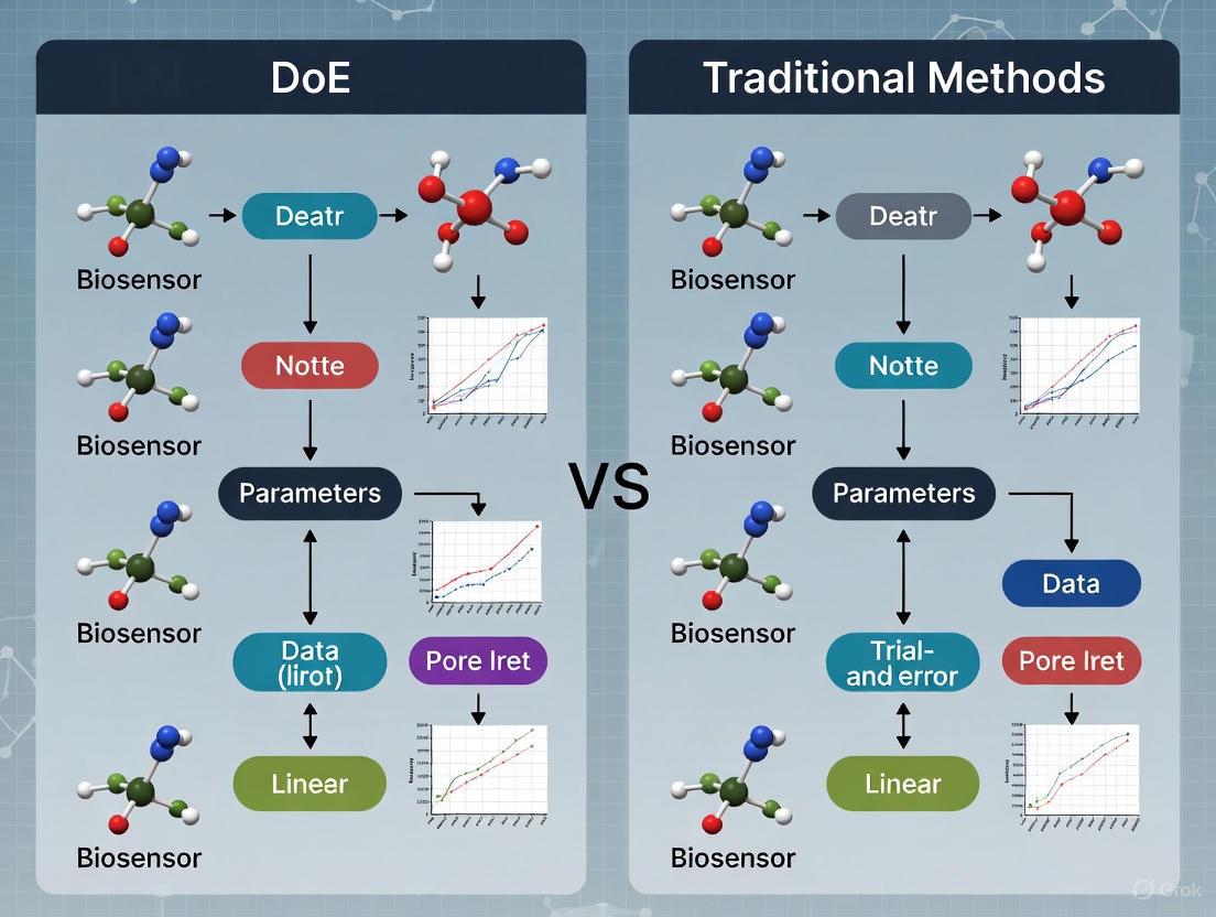
Visualization of Optimization Approaches

The critical need for optimization in ultrasensitive biosensor development cannot be overstated. As biosensors continue to evolve toward greater sensitivity, specificity, and point-of-care applicability, systematic optimization approaches like Design of Experiments provide a fundamental advantage over traditional methods. The comparative analysis demonstrates that DoE methodologies not only enhance biosensor performance but also improve development efficiency, reproducibility, and reliability—all essential factors for successful clinical translation.

Future perspectives in biosensor optimization point toward increased integration of machine learning and artificial intelligence with traditional DoE approaches [4] [7]. The emerging synergy between statistical modeling and AI-driven material informatics holds significant potential for accelerating the discovery of next-generation functional materials and biosensing architectures [7]. Furthermore, the application of explainable AI (XAI) methods provides unprecedented insights into the influence of design parameters, enabling more transparent and interpretable biosensor design processes [4].

As the biosensor field advances toward increasingly complex multi-parameter systems for real-world applications, the systematic optimization principles embodied by DoE will become increasingly indispensable. By bridging the gap between experimental design and computational optimization, these data-driven approaches underscore their transformative impact on enhancing reproducibility, efficiency, and scalability in biosensor research—ultimately accelerating the development of reliable diagnostic tools for improved healthcare outcomes.

The One-Variable-at-a-Time (OVAT) approach, also known as One-Factor-at-a-Time (OFAT), represents a traditional methodology for experimental optimization across scientific and engineering disciplines. This method involves systematically changing a single experimental factor while maintaining all other parameters constant [8]. The OVAT approach has been widely taught and implemented due to its straightforward conceptual framework, which aligns with conventional scientific training [9]. Researchers in fields ranging from biosensor development to pharmaceutical manufacturing have historically relied on this method for optimizing complex processes.

In the specific context of biosensor optimization, which encompasses both manufacturing parameters and operational conditions, the OVAT approach has been frequently employed for initial parameter screening [10]. The method's intuitive nature makes it particularly accessible to non-experts in statistical design, especially in situations where data is relatively inexpensive and abundant to collect [8]. The process begins with establishing baseline conditions for all factors, then sequentially varying each parameter of interest while documenting its individual effect on the output response. This systematic isolation of variables aims to establish clear cause-and-effect relationships between each factor and the measured outcome.

Despite its historical prevalence, the OVAT method faces significant criticism in modern analytical science, particularly when optimizing complex systems with interacting variables [11]. The approach provides only a partial understanding of how factors affect the response, potentially missing optimal conditions and leading to suboptimal system performance [11]. As the demand for more sophisticated and sensitive analytical platforms grows, particularly in fields like biosensor development where multiple manufacturing and operational variables must be optimized simultaneously, understanding the limitations and appropriate applications of OVAT becomes essential for researchers and drug development professionals.

Fundamental Principles and Methodology of OVAT

Core Operational Framework

The OVAT methodology follows a structured, sequential process that can be divided into distinct operational phases. The initial stage involves identifying all potentially relevant factors that may influence the system's output. Researchers then establish baseline conditions for these factors, selecting a starting point that typically represents the current best-known settings or literature values [10]. The optimization process proceeds by selecting one factor to vary across a predetermined range while maintaining all other factors at their baseline levels. After testing each level of the varied factor and measuring the corresponding system response, researchers identify the level that produces the most favorable outcome. This optimal level then becomes the new fixed value for that factor as the process repeats with the next variable [11] [8].

This sequential approach continues until all factors of interest have been individually optimized. The final optimized condition comprises the combination of all individually optimal factor levels identified through this iterative process. The underlying assumption of OVAT is that the global optimum can be approximated by combining the individual optimal levels of each factor, an assumption that holds true only when factors do not interact with each other [12].

Experimental Protocol in Practice

In practical laboratory settings, implementing OVAT requires careful experimental planning and execution. For example, in optimizing pigment production from the marine-derived fungus Talaromyces albobiverticillius 30548, researchers first employed OVAT to screen different nutrient sources [10] [13]. The experimental protocol involved testing five different carbon sources (glucose, sucrose, fructose, soluble starch, and malt extract) while maintaining constant concentrations of nitrogen sources and inorganic salts. After identifying sucrose as the optimal carbon source, researchers then varied nitrogen sources (sodium nitrate, peptone, tryptone, and yeast extract) while maintaining the optimal carbon source and constant inorganic salt concentrations [13].

This systematic approach allowed researchers to identify significant medium components (yeast extract, K₂HPO₄, and MgSO₄·7H₂O) for subsequent optimization phases [10]. The OVAT methodology in this context served as an initial screening tool to narrow down the many potential factors before applying more sophisticated optimization techniques. The stepwise protocol demonstrates how OVAT can provide a foundation for understanding individual factor effects, even in complex biological systems with multiple potential influencing variables.

Figure 1: OVAT Experimental Workflow - This diagram illustrates the sequential process of the One-Variable-at-a-Time approach, showing how factors are optimized individually while others remain constant.

OVAT in Practice: Experimental Applications and Case Studies

Biosensor Optimization Case Study

The application of OVAT in biosensor development demonstrates both the utility and limitations of this approach. In one documented case, researchers developed a paper-based electrochemical biosensor for detecting lung cancer-related microRNAs (miR-155 and miR-21) using an OVAT optimization strategy [11]. The researchers systematically varied parameters such as gold nanoparticle concentration, DNA probe immobilization conditions, ionic strength, and hybridization conditions while keeping other factors constant. This approach enabled preliminary optimization of the sensor, resulting in limits of detection (LODs) of 12.0 nM for miR-155 and 25.7 nM for miR-21 [11].

While this OVAT-based optimization yielded a functional biosensor, the reported detection limits remained relatively high compared to clinical requirements. The authors noted that this highlighted a key drawback of OVAT optimization, which considers only one variable at a time, neglecting possible interactions between factors and often leading to suboptimal performance [11]. Subsequent analysis suggested that had the authors employed a Design of Experiments (DoE) approach, they could have systematically explored the effects of multiple variables simultaneously, potentially identifying synergistic effects and uncovering actual optimal conditions for each parameter [11]. This case illustrates how OVAT can produce functional but potentially suboptimal results in complex biosensor systems where factor interactions may significantly influence performance.

Industrial Bioprocess Optimization

The OVAT approach has also been extensively applied in industrial bioprocess optimization, as demonstrated in pigment production from filamentous fungi. In optimizing pigment production from Talaromyces albobiverticillius 30548, researchers initially employed OVAT to screen different nutrient sources [10]. This involved testing various carbon sources (glucose, sucrose, fructose, soluble starch, and malt extract) while maintaining fixed concentrations of nitrogen sources and inorganic salts. After identifying sucrose as optimal, they then varied nitrogen sources (sodium nitrate, peptone, tryptone, and yeast extract) while maintaining optimal carbon source and constant salts [13].

This OVAT screening identified significant medium components (yeast extract, K₂HPO₄, and MgSO₄·7H₂O) for pigment and biomass production, with sucrose combined with yeast extract providing maximum yields of orange pigments (1.39 g/L) and red pigments (2.44 g/L), along with higher dry biomass (6.60 g/L) [10]. While effective for initial screening, the researchers recognized the limitations of OVAT and subsequently applied Response Surface Methodology (RSM) with Central Composite Design (CCD) to evaluate optimal concentrations and interactive effects between the identified nutrients [10]. This hybrid approach leveraged OVAT for initial factor screening before implementing more sophisticated optimization methodologies, demonstrating a practical application of OVAT within a broader optimization strategy.

Comparative Analysis: OVAT versus Design of Experiments (DoE)

Theoretical Foundations and Operational Differences

The fundamental distinction between OVAT and DoE approaches lies in how they handle multiple variables during experimentation. While OVAT varies factors sequentially while holding others constant, DoE involves systematically varying multiple factors simultaneously according to a predetermined experimental matrix [11] [1]. This fundamental operational difference leads to significant disparities in the type and quality of information obtained from the optimization process.

DoE approaches, including factorial designs, central composite designs, and D-optimal designs, are model-based optimization strategies that develop data-driven models connecting variations in input variables to system outputs [1]. These models enable researchers to not only identify individual factor effects but also quantify interaction effects between factors—something that OVAT approaches cannot accomplish [12]. The ability to detect and measure interactions represents a critical advantage for DoE in complex systems where factors may have interdependent effects on the response variable [11].

Practical Implications for Experimental Efficiency

The efficiency differences between OVAT and DoE become particularly pronounced as the number of experimental factors increases. The table below compares the experimental requirements for OVAT versus various DoE approaches across different numbers of optimization factors:

Table 1: Experimental Requirements Comparison: OVAT vs. DoE Approaches

Number of Factors	OVAT Experiments*	Full Factorial DoE	D-Optimal DoE	Plackett-Burman
3 factors	15-30 experiments	8 experiments	10-15 experiments	4 experiments
6 factors	30-60 experiments	64 experiments	30 experiments	7 experiments
8 factors	40-80 experiments	256 experiments	40-50 experiments	12 experiments

*OVAT experiment estimates assume 5-10 levels tested per factor

A concrete example of this efficiency disparity comes from the development of a hybridization-based paper-based electrochemical biosensor for miRNA-29c detection [11]. The sensing platform involved six variables requiring optimization, including both sensor manufacturing parameters (gold nanoparticles, immobilized DNA probe) and working conditions (ionic strength, probe-target hybridization, electrochemical parameters) [11]. The adoption of a D-optimal DoE design allowed researchers to optimize the device using only 30 experiments, compared to the 486 experiments that would have been required with a comprehensive OVAT approach [11]. This represents a 94% reduction in experimental workload, demonstrating the dramatic efficiency advantages of DoE for multi-factor optimization problems.

Figure 2: Interaction Effects Detection - This diagram illustrates how DoE approaches can identify factor interactions that OVAT methodologies inevitably miss, leading to more comprehensive process understanding.

Performance Outcomes Comparison

The different methodological approaches of OVAT and DoE frequently lead to significantly different optimization outcomes, particularly in complex systems. The table below summarizes performance differences reported in case studies comparing both approaches:

Table 2: Performance Comparison: OVAT vs. DoE Optimization Outcomes

Application Context	OVAT Performance	DoE Performance	Improvement
miRNA electrochemical biosensor [11]	Baseline detection limit	5-fold lower LOD	500% sensitivity improvement
Heavy metal electrochemical sensor [11]	12 nM detection limit	1 nM detection limit	92% sensitivity improvement
Glucose biosensor stability [11]	50% current retention after 12h	75% current retention after 12h	50% stability improvement
Fungal pigment production [10]	6.60 g/L biomass	15.98 g/L biomass	142% yield improvement

The performance advantages of DoE are particularly evident in the miRNA biosensor case study, where adopting a D-optimal DoE design resulted in a 5-fold improvement in the limit of detection compared to the non-DoE optimized biosensor [11]. Similarly, in optimizing an electrochemical glucose biosensor, DoE enabled researchers to achieve similar current density using 93% less nanoconjugate while improving operational stability from 50% to 75% amperometric current retained after 12 hours of use [11]. These performance improvements stem from DoE's ability to identify true optimal conditions by accounting for factor interactions, which OVAT approaches inherently cannot detect.

The Researcher's Toolkit: Essential Materials and Reagents

Successful implementation of OVAT optimization requires specific research tools and reagents tailored to the experimental context. The following table outlines key materials commonly employed in OVAT-based biosensor optimization studies:

Table 3: Essential Research Reagents for Biosensor Optimization Studies

Reagent/Material	Function in Optimization	Application Example
Gold nanoparticles	Signal amplification in electrochemical biosensors	Varied concentration to enhance electron transfer [11]
DNA probes	Biorecognition element for nucleic acid detection	Immobilization density optimized for target hybridization [11]
Yeast extract	Complex nitrogen source for microbial growth	Optimized as nitrogen source for fungal pigment production [10]
MgSO₄·7H₂O	Enzyme cofactor and metabolic precursor	Concentration optimized for fungal metabolite production [10]
Screen-printed electrodes	Transduction platform for electrochemical detection	Surface modification parameters optimized sequentially [14]
Carbon nanotubes	Nanomaterial for electrode modification	Loading concentration optimized for signal enhancement [14]

These fundamental materials represent core components across many biosensor optimization studies. Their concentrations, immobilization parameters, and processing conditions are typically varied sequentially in OVAT approaches to establish individual optimal ranges before proceeding to subsequent factors. The selection of appropriate ranges for each variable requires preliminary knowledge of the system, which may come from literature reviews, preliminary experiments, or theoretical considerations [10].

Critical Assessment: Advantages and Limitations of OVAT

Documented Advantages in Specific Contexts

Despite its methodological limitations, the OVAT approach maintains relevance in certain research contexts due to several distinct advantages. The method is conceptually straightforward and widely taught, making it accessible to researchers without extensive statistical training [9]. This accessibility particularly benefits non-experts and those entering new research fields where preliminary factor screening is necessary [8]. The logical progression of varying one factor at a time aligns with conventional scientific thinking about cause-and-effect relationships, making experimental procedures and results intuitively understandable to broad audiences.

OVAT approaches demonstrate particular utility in situations where data is relatively inexpensive and abundant to collect [8]. In early-stage exploratory research, where little prior knowledge exists about factor effects, OVAT can provide initial insights with minimal statistical analysis requirements. Some researchers have shown that OVAT can be more effective than fractional factorial designs under specific conditions: when the number of experimental runs is severely limited, the primary goal is to attain incremental improvements in the system, and experimental error is not large compared to factor effects (which must be additive and independent of each other) [8]. Additionally, OVAT serves as a valuable preliminary step before implementing more sophisticated DoE approaches, helping to identify critical factors for subsequent comprehensive optimization [10].

Fundamental Limitations and Methodological Flaws

The OVAT approach suffers from several fundamental limitations that restrict its effectiveness for complex optimization challenges. The most significant drawback is its inability to detect and quantify interactions between factors [11] [12]. When factors interact—meaning the effect of one factor depends on the level of another—OVAT may completely miss the true optimal conditions, potentially identifying suboptimal parameter combinations [11]. This limitation is particularly problematic in biosensor optimization, where interactions between manufacturing parameters (e.g., nanomaterial concentration) and operational conditions (e.g., ionic strength, temperature) are common.

Additional limitations include inefficiency in resource utilization, as OVAT requires more experimental runs for the same precision in effect estimation compared to statistically designed experiments [8] [9]. The method provides limited coverage of the experimental space, focusing on axial points while potentially missing optimal regions located elsewhere in the multidimensional factor space [9]. There is also no inherent mechanism to account for or quantify experimental error, including measurement variation, which makes it difficult to determine the statistical significance of observed effects [12]. These collective limitations explain why OVAT has been largely superseded by DoE methodologies in fields requiring rigorous optimization of complex multi-factor systems, particularly in biosensor development and pharmaceutical applications [11] [1].

The One-Variable-at-a-Time approach represents a foundational methodology in experimental optimization with specific utilities and recognized limitations. While its straightforward conceptual framework makes it accessible for preliminary factor screening and educational contexts, OVAT suffers from critical drawbacks in complex optimization scenarios, particularly its inability to detect factor interactions and its inefficiency in resource utilization [11] [8] [12]. The demonstrated performance advantages of Design of Experiments approaches—including 5-fold improvements in detection limits for biosensors and substantial reductions in experimental workload—highlight why DoE methodologies have largely superseded OVAT in rigorous scientific optimization [11].

Nevertheless, OVAT maintains relevance as an initial screening tool within broader optimization strategies, particularly when researchers possess limited prior knowledge about a system [10]. The method's accessibility ensures its continued application in early-stage research, though scientists should recognize its limitations and transition to more sophisticated DoE approaches for comprehensive optimization. For researchers and drug development professionals working with complex systems like biosensors, where multiple interacting factors influence performance outcomes, understanding both the appropriate applications and fundamental limitations of OVAT remains essential for designing efficient and effective optimization strategies.

In the field of biosensor development and drug discovery, efficient experimental optimization is crucial for advancing new technologies from concept to clinical application. The traditional One-Variable-at-a-Time (OVAT) approach has been widely used for process optimization, but it possesses fundamental limitations that can hinder research progress and outcomes. This guide examines these inherent constraints through direct comparison with the statistical approach of Design of Experiments (DoE), supported by experimental data and case studies from recent scientific literature.

OVAT vs. DoE: A Fundamental Comparison

OVAT (One-Variable-at-a-Time), also known as OFAT, is an experimental approach where researchers test factors individually while holding all other variables constant [8] [15]. After testing one factor, they return it to its baseline before investigating the next variable. This method has historically been popular due to its conceptual simplicity and straightforward implementation [15].

DoE (Design of Experiments) is a systematic, statistical approach that involves varying multiple factors simultaneously according to a predefined experimental matrix [16]. This methodology enables researchers to not only determine individual factor contributions but also to resolve factor interactions and create detailed maps of process behavior.

Table: Fundamental Methodological Differences Between OVAT and DoE

Aspect	OVAT Approach	DoE Approach
Factor Variation	Factors tested sequentially	Multiple factors varied simultaneously
Interaction Detection	Cannot estimate interactions	Can resolve and quantify factor interactions
Experimental Efficiency	Requires more runs for same precision	More information with fewer experiments
Optima Identification	Prone to finding local optima	Better at identifying global optima
Error Estimation	Requires multiple replicates	Uses centerpoints to estimate pure error

Core Limitations of the OVAT Approach

Experimental Inefficiency and Resource Intensity

The OVAT method requires a substantially larger number of experimental runs to achieve the same precision in effect estimation compared to factorial designs [8] [15]. This inefficiency stems from its sequential nature, where each variable must be tested individually while others remain fixed. In chemical reaction optimization, this approach is "simple but laborious and time consuming, requiring many individual runs across an often-large number of parameters" [16]. The increased number of runs directly translates to higher consumption of reagents, expensive materials, and researcher time—particularly problematic when working with precious samples or specialized equipment.

Inability to Detect Factor Interactions

Perhaps the most significant limitation of OVAT is its fundamental inability to detect interactions between factors [8] [15]. By varying only one factor at a time, OVAT assumes that factors act independently, which is often an unrealistic assumption in complex biological and chemical systems.

As demonstrated in radiochemistry optimization, "the setting of one factor may affect the influence of another" [16]. These interaction effects can be crucial in biosensor development, where parameters like pH, temperature, and reagent concentrations often exhibit interdependent effects on sensor performance. Without detecting these interactions, researchers risk drawing incomplete or misleading conclusions about their systems.

Propensity to Identify Local Rather Than Global Optima

OVAT optimization is "prone to finding only local optima" and may "miss the true set of optimal conditions" [16]. This occurs because the method only explores a limited path through the experimental space rather than mapping the entire response surface. The results are highly dependent on the starting conditions chosen by the researcher, potentially leading to suboptimal outcomes that don't represent the best possible configuration for a given biosensor or chemical process.

Case Studies and Experimental Evidence

Radiochemistry Optimization: DoE vs. OVAT Efficiency

In copper-mediated radiofluorination (CMRF) chemistry for PET tracer synthesis, researchers directly compared DoE and OVAT approaches [16]. Using DoE to construct factor screening and optimization studies, they "identified critical factors and modeled their behavior with more than two-fold greater experimental efficiency than the traditional OVAT approach." This enhanced efficiency is particularly valuable in radiochemistry, where reducing experimental runs lowers researcher exposure to ionizing radiation and conserves expensive precursors.

Table: Experimental Efficiency Comparison in Radiochemistry Optimization

Metric	OVAT Approach	DoE Approach	Improvement
Experimental Runs	Substantially more required	Minimized via statistical design	>2x more efficient
Interaction Detection	Not possible	Full resolution of factor interactions	Critical insights gained
Optimal Condition Identification	Local optima likely	Global optima identified	Enhanced process performance
Resource Consumption	High	Optimized	Significant savings

Biosensor Performance Optimization

Recent advances in biosensor development have leveraged DoE and machine learning to overcome OVAT limitations. In developing a photonic crystal fiber surface plasmon resonance (PCF-SPR) biosensor, researchers integrated "machine learning regression techniques to predict key optical properties" and "explainable AI methods to analyze model outputs and identify the most influential design parameters" [17]. This hybrid approach "significantly accelerates sensor optimization, reduces computational costs, and improves design efficiency compared to conventional methods."

Similarly, in optimizing a graphene-based biosensing platform for breast cancer detection, machine learning models were used to "systematically optimize structural parameters, enabling systematic refinement of detection accuracy and reproducibility" [18]. The optimized design demonstrated superior sensitivity compared to conventional configurations, achieving "a peak sensitivity of 1785 nm/RIU."

Recommended Experimental Protocols

DoE Factor Screening Protocol

For initial DoE implementation in biosensor optimization:

• Define Objective: Clearly identify the primary response variable (e.g., sensitivity, specificity, signal-to-noise ratio).

• Select Factors: Choose continuous (temperature, pH, concentration) and discrete (buffer type, membrane material) variables based on preliminary knowledge.

• Design Screening Experiment: Implement a fractional factorial design to efficiently identify significant factors from a larger set of potential variables [16].

• Execute and Analyze: Conduct experiments according to the design matrix, then use multiple linear regression to identify statistically significant factors.

• Plan Optimization Phase: Use significant factors identified in screening to design more detailed response surface optimization studies.

Response Surface Methodology Protocol

For detailed optimization after factor screening:

• Select Experimental Design: Choose central composite or Box-Behnken designs capable of modeling curvature and interactions [15].

• Execute Design: Perform experiments across the defined factor space, including center points for error estimation.

• Model Development: Fit a mathematical model (typically quadratic) to the response data using regression analysis.

• Optimization: Use the fitted model to identify factor settings that optimize the response(s).

• Validation: Confirm optimal conditions through additional experimental runs.

Research Reagent Solutions for Optimization Studies

Table: Essential Materials for Biosensor Optimization Experiments

Reagent/Material	Function in Optimization	Application Examples
Graphene-based composites	Enhanced sensitivity and conductivity	Breast cancer biosensors [18]
Gold/Silver nanoparticles	Plasmonic enhancement	SERS-based immunoassays [19]
Photonic crystal fibers	Light propagation control	PCF-SPR biosensors [17]
Specific antibodies	Target recognition	α-fetoprotein detection [19]
Fluorescent dyes	Signal generation and detection	Various immunoassays
Buffer components	pH maintenance and stability	All biological assays

The inherent limitations of OVAT—local optima identification, missed factor interactions, and experimental inefficiency—present significant challenges in biosensor optimization and drug development. The demonstrated superiority of DoE approaches in both efficiency and effectiveness underscores the value of statistical experimental design in modern research. As the field advances, integrating DoE with emerging technologies like machine learning and explainable AI provides a powerful framework for accelerating development cycles and enhancing diagnostic capabilities in biomedical applications.

The development of high-performance biosensors represents a critical frontier in medical diagnostics, environmental monitoring, and biotechnology. However, the transition from laboratory prototypes to reliable, commercially viable sensing platforms has been consistently hampered by optimization challenges [1]. Traditional one-variable-at-a-time (OVAT) approaches to biosensor optimization—where parameters are adjusted sequentially while others remain fixed—suffer from fundamental limitations in efficiently navigating complex, multidimensional experimental spaces [1] [2]. This comparative analysis examines Design of Experiments (DoE) as a systematic framework for biosensor optimization, contrasting its methodology and performance against traditional approaches with supporting experimental data.

Design of Experiments is a powerful chemometric tool that provides a structured, model-based approach to optimization [1] [2]. Unlike traditional methods, DoE simultaneously varies multiple experimental factors according to predetermined mathematical matrices, enabling researchers to not only determine individual variable effects but also to identify interaction effects between variables—a capability that consistently eludes OVAT approaches [1]. This perspective review demonstrates how DoE methodologies have been successfully applied to optimize both optical and electrical ultrasensitive biosensors, resulting in enhanced performance metrics including sensitivity, dynamic range, and signal-to-noise ratios while reducing overall experimental effort [1] [2].

Traditional OVAT Optimization: Limitations and Pitfalls

Fundamental Methodological Flaws

The traditional OVAT approach to biosensor optimization follows a sequential process wherein individual parameters such as bioreceptor concentration, cross-linking agent amount, pH, or temperature are optimized independently while other variables remain fixed at arbitrary levels [1]. This method appears logically straightforward but contains critical statistical and practical deficiencies that limit its effectiveness for complex biosensing systems.

The most significant limitation of OVAT methodology is its inherent inability to detect interaction effects between variables [1] [2]. In biosensor systems, interaction effects occur when the influence of one factor (e.g., enzyme concentration) on the response (e.g., signal intensity) depends on the level of another factor (e.g., pH). These interactions are particularly common in complex biological systems but remain completely undetectable through OVAT experimentation [1]. Consequently, conditions established through sequential optimization may not represent the true global optimum, potentially leading to suboptimal biosensor performance in practical applications [1] [2].

Practical Consequences for Biosensor Development

From a practical standpoint, OVAT optimization often leads to increased experimental effort, higher resource consumption, and prolonged development timelines [20]. While each individual OVAT experiment might appear efficient, the cumulative number of experiments required to explore multiple factors often exceeds the more economical experimental matrices employed in DoE [1]. Furthermore, the localized knowledge gained through OVAT provides limited understanding of the overall experimental domain, offering little predictive capability beyond the specifically tested conditions [1].

Recent studies highlight how traditional optimization approaches have hindered biosensor development. For enzymatic glucose biosensors, conventional optimization of parameters including enzyme amount, cross-linker concentration, conducting polymer properties, and measurement conditions has typically required extensive experimental setups and fabrication of numerous biosensors under different conditions [20]. This chemometric approach inevitably increases both cost and time consumption during the sensor design phase [20].

DoE Methodology: A Systematic Framework

Theoretical Foundations and Core Principles

Design of Experiments represents a fundamental shift from traditional optimization approaches by employing structured, statistically-based experimental matrices that efficiently explore multiple factors simultaneously [1] [2]. The DoE workflow begins with identifying all factors that may exhibit causal relationships with the targeted output signal (response) [1]. After factor selection, researchers establish experimental ranges and determine the distribution of experiments within the experimental domain [1].

The responses collected from these predetermined points are used to construct mathematical models through linear regression, elucidating the relationship between experimental conditions and outcomes [1]. Unlike OVAT's localized knowledge, DoE enables response prediction at any point within the experimental domain, providing comprehensive, global understanding of the system [1]. This approach not only offers significant empirical value but also yields data-driven models that can provide insights into the physical rationalization of observed effects, frequently offering valuable and unforeseen understanding of fundamental mechanisms underlying transduction and amplification processes [1].

Key Experimental Designs for Biosensor Optimization

Table 1: Common Experimental Designs in Biosensor Optimization

Design Type	Experimental Requirements	Model Capability	Key Applications	Advantages
Full Factorial	2k experiments for k factors [1]	First-order effects and interactions [1]	Initial screening of multiple factors [1]	Identifies all interaction effects; orthogonal design [1]
Central Composite	Augmented factorial design with center and axial points [1]	Second-order (quadratic) effects [1]	Response surface modeling and optimization [1]	Captures curvature in response; enables location of optima [1]
Mixture Design	Specialized for composition variables [1]	Component proportion effects [1]	Formulation optimization with constrained components [1]	Accounts for dependency between components (sum to 100%) [1]
Definitive Screening	Highly efficient for many factors [21]	Main effects and some interactions [21]	Systems with numerous potential factors [21]	Requires minimal runs; robust to active factor sparsity [21]

Implementation Workflow

The implementation of DoE follows a systematic workflow that differs fundamentally from traditional approaches. The process typically involves multiple iterative cycles of design-build-test-learn, with no more than 40% of available resources allocated to the initial set of experiments [1]. Subsequent iterations use data from initial designs to refine the problem by eliminating insignificant variables, redefining experimental domains, or adjusting hypothesized models [1].

Diagram 1: DoE Iterative Workflow. The systematic process for implementing Design of Experiments emphasizes iterative refinement and model validation to reach optimal conditions efficiently.

Comparative Performance Analysis: DoE vs. Traditional Methods

Case Study: Whole Cell Biosensor Optimization

A definitive comparative study demonstrated the superior performance of DoE over traditional methods in optimizing whole-cell biosensors for detecting catabolic breakdown products of lignin biomass [21]. Researchers applied DoE methodology to systematically modify biosensor dose-response behavior by exploring multidimensional experimental space with minimal experimental runs [21].

Table 2: Performance Comparison for Whole Cell Biosensor Optimization

Performance Metric	Traditional Methods	DoE Approach	Improvement Factor
Maximum Signal Output	Baseline	Up to 30-fold increase [21]	30×
Dynamic Range	Baseline	>500-fold improvement [21]	>500×
Sensing Range	Limited	Expanded by ~4 orders of magnitude [21]	10,000×
Sensitivity	Baseline	>1500-fold increase [21]	>1,500×
Dose-Response Modulation	Fixed response	Digital and analogue behavior achievable [21]	N/A
Experimental Efficiency	Resource-intensive iterative cycles [21]	Structured exploration with minimal runs [21]	Significant reduction

The study demonstrated that DoE could efficiently map experimental space and develop genetic systems with greatly enhanced output signal, basal control, dynamic range, and sensitivity compared to standard iterative approaches [21]. The methodology enabled researchers to convert different, closely related genetic designs into continuous factors, avoiding the need to repeat all experimental conditions for each genetic design [21].

Case Study: Electrochemical Biosensor Optimization

Research on electrochemical biosensors further demonstrates DoE advantages. Traditional optimization of enzymatic glucose biosensors requires extensive experimentation to optimize parameters including enzyme amount, cross-linker concentration (e.g., glutaraldehyde), conducting polymer scan number, and measurement conditions [20]. This process necessitates fabricating numerous biosensors with different conditions, increasing both cost and development time [20].

Machine learning approaches applied to biosensor optimization have revealed complex, nonlinear relationships between fabrication parameters and electrochemical responses that traditional OVAT approaches would struggle to identify [20]. These relationships include interaction effects between factors such as enzyme loading, pH, and cross-linker concentration that significantly impact biosensor performance but remain undetectable through sequential optimization [20].

DoE Experimental Protocols and Implementation

Protocol 1: Full Factorial Design for Initial Screening

Objective: Identify significant factors and two-factor interactions affecting biosensor response [1].

Methodology:

• Select k factors for initial screening (typically 3-5 key parameters)
• Define low (-1) and high (+1) levels for each factor based on preliminary knowledge
• Construct 2k experimental matrix with coded factor levels [1]
• Randomize run order to minimize systematic bias
• Conduct experiments and record responses (e.g., signal intensity, limit of detection)
• Compute model coefficients using least squares method [1]
• Perform statistical analysis to identify significant effects and interactions

Mathematical Model: For a 2^2 factorial design, the model takes the form: Y = b0 + b1X1 + b2X2 + b12X1X2, where Y is the predicted response, b0 is the intercept, b1 and b2 are main effects, and b12 is the interaction effect [1].

Protocol 2: Central Composite Design for Response Optimization

Objective: Model curvature in response surface and locate optimal conditions [1].

Methodology:

• Begin with factorial design points (2k)
• Add center points (typically 3-6) to estimate pure error
• Add axial (star) points at distance ±α from center to estimate quadratic effects
• The total number of experiments = 2k + 2k + C0, where C0 is the number of center points
• Conduct experiments in randomized order
• Fit second-order model using regression analysis
• Validate model with confirmation experiments at predicted optimum

Application: This design is particularly valuable when the response follows a quadratic function with respect to experimental variables, allowing precise location of optimal conditions [1].

The Scientist's Toolkit: Essential Research Reagents and Materials

Table 3: Key Research Reagents for Biosensor Optimization Studies

Reagent/Material	Function in Optimization	Application Examples
Glutaraldehyde	Cross-linking agent for enzyme immobilization [20]	Covalent binding of enzymes to nanomaterials; creates robust enzyme-substrate interaction [22]
N-Hydroxysuccinimide (NHS)/EDC	Carboxyl group activation for covalent bonding [19]	Functionalization steps for antibody attachment on sensor surfaces [19]
Gold Nanoparticles	Signal amplification and enhanced electron transfer [22]	Improving electrochemical response in immunosensors; increased surface area for biorecognition element immobilization [22]
Graphene & MXenes	Nanomaterials with high conductivity and surface area [20] [23]	Enhancing sensitivity in electrochemical and optical biosensors; Femtomolar-level detection [20]
Polydopamine	Versatile surface coating material [19]	Improving biocompatibility and facilitating functionalization through simple, environmentally friendly procedures [19]
Enzyme Solutions	Biological recognition elements [20]	Glucose oxidase, horseradish peroxidase, and other enzymes for specific analyte detection [20]

Integration with Advanced Computational Methods

Machine Learning and DoE Synergy

Recent advances combine DoE with machine learning (ML) approaches to further enhance biosensor optimization. ML algorithms can model complex, nonlinear relationships between fabrication parameters and biosensor responses that may challenge traditional DoE models [20]. Studies have demonstrated that ML regression techniques can accurately predict biosensor performance based on key input parameters, potentially reducing experimental burden [20] [23].

The integration of explainable AI (XAI) methods, particularly Shapley Additive exPlanations (SHAP), with DoE provides enhanced interpretability of model outputs, helping researchers identify the most influential design parameters [23]. This hybrid approach significantly accelerates sensor optimization, reduces computational costs, and improves design efficiency compared to conventional methods [23].

Comparative Workflow Efficiency

Diagram 2: Workflow Comparison. Contrast between traditional OVAT (left) and DoE (right) approaches highlights DoE's parallel experimentation and model-based optimization versus OVAT's sequential process.

The comparative analysis clearly demonstrates that Design of Experiments provides a superior framework for biosensor optimization compared to traditional OVAT approaches. DoE systematically uncovers factor interactions, reduces experimental effort, and enables global optimization through structured experimentation and mathematical modeling [1] [2] [21]. The documented performance improvements across multiple biosensor platforms—including whole-cell, electrochemical, and optical biosensors—confirm the practical value of this methodology [1] [21] [23].

Future developments in biosensor optimization will likely involve tighter integration between DoE and machine learning approaches, leveraging the strengths of both methodologies [20] [23]. The growing application of explainable AI will further enhance interpretability, providing deeper insights into the fundamental relationships between design parameters and biosensor performance [23]. As biosensor technologies continue to advance toward increasingly complex multiplexed systems and point-of-care applications, the systematic framework offered by DoE will become increasingly essential for efficient development and optimization.

For researchers engaged in biosensor development, adopting DoE methodologies represents not merely a statistical improvement but a fundamental paradigm shift that accelerates development cycles, enhances performance, and provides deeper understanding of the complex systems under investigation. The experimental evidence and comparative data presented in this analysis provide a compelling case for implementing DoE as the standard approach for biosensor optimization across diverse applications and technology platforms.

In the field of biosensor development, researchers and drug development professionals face the constant challenge of creating devices with enhanced sensitivity, specificity, and reliability. Traditional optimization methods, particularly the "one factor at a time" (OFAT) approach, have shown significant limitations in efficiently navigating the complex multidimensional experimental spaces inherent to biosensor systems [1]. OFAT methodologies involve varying a single parameter while holding all others constant, which not only proves inefficient but more critically, fails to detect interactions between factors that can profoundly influence biosensor performance [24] [25].

Design of Experiments (DoE) provides a powerful, systematic framework that overcomes these limitations through structured multivariate experimentation [24]. DoE is a branch of applied statistics that deals with planning, conducting, analyzing, and interpreting controlled tests to evaluate the factors that control the value of a parameter or group of parameters [24]. By simultaneously manipulating multiple input factors according to statistically designed matrices, DoE enables researchers to efficiently identify optimal conditions while quantifying both main effects and interaction effects [26]. This approach is particularly valuable for optimizing complex genetic systems in biosensor development, where multiple protein-protein and protein-DNA interactions often display nonlinear effects that OFAT approaches cannot adequately characterize [21].

The following comparison guide examines the core principles of DoE, with specific focus on factorial designs and response surface methodology, and demonstrates how these approaches provide superior optimization capabilities compared to traditional methods for biosensor development.

Fundamental DoE Principles and Their Strategic Advantages

Core Principles of DoE

The foundation of DoE rests upon three key principles that ensure the validity and reliability of experimental results: randomization, replication, and blocking [27] [24].

• Randomization: This principle involves the random assignment of experimental runs to different factor level combinations. Randomization helps mitigate the impact of nuisance variables and ensures that any observed effects can be attributed to the factors under investigation rather than uncontrolled sources of variation. In comparative experiments, such as evaluating treatments versus controls, random assignment of treatments is essential for eliminating potential biases from conclusions [27].

• Replication: Replication refers to the repetition of complete experimental treatments, including the setup. This practice allows researchers to estimate the inherent variability in the experimental process and provides a measure of experimental error. Through replication, researchers can determine the precision of their estimates and obtain more reliable results [27] [24].

• Blocking: Blocking is a technique used to account for known sources of variability in an experiment, such as differences in equipment, operators, or environmental conditions. By grouping experimental runs into homogeneous blocks, researchers can isolate and quantify the effects of these nuisance variables, leading to more precise estimates of the factor effects of primary interest [27] [26].

DoE Versus Traditional OFAT: A Comparative Analysis

The table below summarizes the key differences between the traditional OFAT approach and the structured DoE methodology:

Table 1: Comparison between OFAT and DoE Methodologies

Aspect	OFAT (Traditional Approach)	DoE (Systematic Approach)
Experimental Strategy	Varies one factor while holding others constant	Varies multiple factors simultaneously according to statistical design
Interaction Detection	Cannot detect interactions between factors	Explicitly models and quantifies factor interactions
Efficiency	Inefficient; requires many experiments for few factors	Highly efficient; explores large experimental spaces with minimal runs
Model Building	Limited to first-order understanding	Enables building of predictive mathematical models
Optimal Condition Identification	May miss true optimum due to ignored interactions	Systematically locates optimal regions and identifies trade-offs
Biosensor Application	Problematic for complex systems with interacting components	Ideal for optimizing multifactorial biosensor systems

Traditional OFAT approaches are inherently limited because they fail to capture interactions between factors. For instance, in biosensor development, the effect of changing an immobilization pH might depend on the temperature or ionic strength of the solution. OFAT would miss this critical dependency, potentially leading researchers to suboptimal configurations [1] [24].

In contrast, DoE approaches not only identify significant main effects but also quantify how factors interact. This capability is particularly valuable in biosensor optimization, where factors such as biorecognition element concentration, immobilization time, and detection conditions often exhibit complex interdependencies that significantly impact the final biosensor performance in terms of sensitivity, dynamic range, and limit of detection [1].

Factorial Designs: Screening and Evaluating Factors

Fundamentals of Factorial Designs

Factorial designs form the backbone of many DoE investigations, particularly in the initial stages of biosensor optimization. These designs involve studying the effects of multiple factors simultaneously by investigating all possible combinations of the factor levels [26]. The most basic factorial design is the 2-level full factorial, denoted as 2^k, where k represents the number of factors being studied, with each factor tested at two levels (typically coded as -1 and +1) [1].

The key advantage of factorial designs lies in their ability to estimate not only the main effects of each factor (the average change in response when a factor moves from its low to high level) but also the interaction effects between factors (how the effect of one factor depends on the level of another factor) [26]. This comprehensive assessment of both main and interaction effects enables researchers to develop a more complete understanding of their biosensor system than would be possible with OFAT approaches.

Types of Factorial Designs

Full factorial designs investigate all possible combinations of factors and levels, providing complete information on main effects and all orders of interactions. However, the number of experimental runs required for a full factorial design grows exponentially with the number of factors (2^k for a 2-level design), which can become resource-prohibitive when studying many factors [26] [25].

Fractional factorial designs address this limitation by strategically investigating only a subset (fraction) of the full factorial combinations. These designs operate on the principle of sparsity of effects, assuming that while there may be many possible effects, only a few (typically main effects and two-factor interactions) are likely to be important [25]. Although fractional factorial designs require fewer runs, this efficiency comes at the cost of aliasing, where certain effects cannot be distinguished from one another [25].

Table 2: Types of Factorial Designs and Their Characteristics

Design Type	Number of Runs	Information Obtained	Best Use Cases
Full Factorial	2^k (for 2-level designs)	All main effects and all interactions	When number of factors is small (typically ≤5) and resources allow
Fractional Factorial	2^(k-p) (where p represents the fraction)	Main effects and lower-order interactions, but with aliasing	Screening many factors (typically >5) with limited resources
Mixed-Level Factorial	Varies based on level combinations	Effects of both categorical and continuous factors	When experimenting with different types of factors simultaneously

Application in Biosensor Optimization

Factorial designs have proven particularly valuable in biosensor optimization. For example, in the development of whole-cell biosensors for detecting catabolic breakdown products of lignin biomass, researchers utilized a definitive screening design to efficiently map the experimental space by systematically modifying genetic components [21]. Through this approach, they successfully enhanced biosensor performance by increasing maximum signal output (up to 30-fold), improving dynamic range (>500-fold), expanding sensing range (approximately 4 orders of magnitude), and increasing sensitivity (by >1500-fold) compared to initial configurations [21].

The following diagram illustrates a typical workflow for applying factorial designs in biosensor optimization:

Response Surface Methodology: Modeling and Optimization

Fundamentals of Response Surface Methodology

Once significant factors have been identified through factorial designs, Response Surface Methodology (RSM) provides a powerful collection of statistical and mathematical techniques for modeling and optimization [28] [29]. RSM uses regression analysis to fit empirical models to experimental data, enabling researchers to locate optimal conditions within the experimental region [28].

The primary goal of RSM is to efficiently navigate the experimental space to identify factor settings that produce the best possible response values, whether the objective is to maximize, minimize, or achieve a target value [29]. This approach is particularly valuable in biosensor optimization, where multiple performance characteristics (e.g., sensitivity, dynamic range, specificity) must often be balanced simultaneously.

RSM typically employs sequential experimentation, beginning with first-order models for initial exploration and progressing to second-order models that can capture curvature in the response surface [29]. The general form of a second-order response surface model for k factors is:

[ y = \beta0 + \sum{i=1}^k \betai xi + \sum{i=1}^k \beta{ii} xi^2 + \sum{i{ij} xi x_j + \varepsilon ]

Where y represents the predicted response, β₀ is the constant term, βi represents the coefficients for linear effects, βii represents the coefficients for quadratic effects, β_ij represents the coefficients for interaction effects, and ε represents the random error [28] [29].

Key RSM Designs

Several specialized experimental designs have been developed specifically for response surface methodology:

• Central Composite Designs (CCD): These designs consist of a two-level factorial or fractional factorial component (2^k) augmented with center points and axial (star) points [30] [31]. The axial points allow estimation of curvature, making CCDs appropriate for fitting second-order models. CCDs can be made rotatable through careful selection of the axial point distance (α), meaning the prediction variance depends only on the distance from the design center and not on direction [30] [31].

• Box-Behnken Designs: These are spherical, rotatable designs that consist of combinations of factor levels at the midpoints of the edges of the experimental space and center points [30]. Box-Behnken designs are often more efficient than CCDs when the corners of the experimental space are expensive or impossible to reach.

The diagram below illustrates the structure of a central composite design for two factors:

Implementation of RSM

The implementation of RSM typically follows a structured sequence:

• Problem Definition: Clearly define the optimization objectives and identify the critical response variables that characterize biosensor performance (e.g., limit of detection, signal-to-noise ratio, dynamic range) [28].

• Factor Screening: Use factorial designs to identify the most influential factors from a larger set of potential variables [28] [25].

• Experimental Design Selection: Choose an appropriate RSM design (e.g., CCD, Box-Behnken) based on the number of factors, resources available, and suspected complexity of the response surface [30].

• Model Development: Conduct experiments according to the design matrix and use regression analysis to fit an appropriate response surface model to the data [28].

• Model Validation: Check the adequacy of the fitted model using statistical tests (e.g., ANOVA, lack-of-fit tests) and residual analysis [28] [30].

• Optimization: Use the validated model to locate optimal factor settings through techniques such as canonical analysis or numerical optimization [28] [29].

• Confirmation: Conduct confirmation experiments at the predicted optimal conditions to verify model predictions [28].

Comparative Experimental Data: DoE vs Traditional Methods

Quantitative Performance Comparison

The superiority of DoE approaches over traditional OFAT methods is demonstrated through quantitative performance metrics across various optimization studies. The table below summarizes experimental data comparing the two approaches in biosensor optimization:

Table 3: Performance Comparison of DoE vs OFAT in Biosensor Optimization

Performance Metric	OFAT Optimization	DoE Optimization	Improvement Factor
Maximum Signal Output	Baseline	Up to 30-fold increase	30x [21]
Dynamic Range	Baseline	>500-fold improvement	>500x [21]
Sensing Range	Baseline	~4 orders of magnitude expansion	~10,000x [21]
Sensitivity	Baseline	>1500-fold increase	>1500x [21]
Experimental Effort	High (many sequential experiments)	Significantly reduced	~50-80% reduction [1]
Interaction Detection	Not possible	Comprehensive mapping of factor interactions	N/A [24]

Case Study: Whole-Cell Biosensor Optimization

A compelling example of DoE application in biosensor development comes from research on whole-cell biosensors for detecting catabolic breakdown products of lignin biomass [21]. Researchers applied a definitive screening design to optimize a protocatechuic acid (PCA)-responsive biosensor by systematically modifying three genetic factors: the promoter regulating the transcription factor (Preg), the output promoter (Pout), and the ribosome binding site controlling reporter expression (RBSout) [21].

The DoE approach enabled the researchers to efficiently explore the multidimensional experimental space and identify optimal combinations of genetic components that would have been virtually impossible to discover using OFAT. The resulting optimized biosensors exhibited dramatically improved performance characteristics, including both "digital" biosensors with sharp, switch-like dose-response behavior for clear binary classification and "analogue" biosensors with graded responses for quantifying analyte concentration over a wide range [21].

This case study illustrates how DoE not only enhances traditional biosensor performance metrics but also enables the engineering of novel response modalities that can be tailored to specific application requirements.

Essential Research Reagent Solutions for DoE Implementation

Successful implementation of DoE in biosensor optimization requires specific research reagents and materials. The following table details key solutions and their functions:

Table 4: Essential Research Reagent Solutions for DoE in Biosensor Optimization

Reagent/Material	Function in DoE	Application Examples
Statistical Software Packages	Experimental design generation, data analysis, model fitting, and optimization	JMP, Minitab, Design-Expert, R with DoE packages [24] [31]
Coded Variable Templates	Standardization of factor levels across different measurement scales	Excel templates with pre-coded factor levels (-1, 0, +1) [24]
High-Throughput Screening Systems	Efficient execution of multiple experimental runs under controlled conditions	Automated liquid handling systems, multi-well plate readers [21]
Standardized Buffer Systems	Control of environmental factors during biosensor testing and characterization	pH buffers, ionic strength solutions, temperature control systems [1]
Reference Materials & Calibrants	Validation of measurement systems and response assessment	Certified reference materials, standard solutions for calibration [1]
Quality Control Samples	Monitoring of experimental process stability and variance estimation	Replicate samples, control charts for response measurement [27]

The comparison between traditional OFAT approaches and systematic DoE methodologies reveals significant advantages for factorial designs and response surface methodology in biosensor optimization. Through their ability to efficiently explore complex experimental spaces, quantify factor interactions, and build predictive models, DoE approaches enable researchers to achieve performance enhancements that are difficult or impossible to attain with traditional methods.

The experimental data demonstrates that DoE can deliver order-of-magnitude improvements in key biosensor performance metrics, including signal output, dynamic range, sensing range, and sensitivity, while simultaneously reducing experimental effort. Furthermore, the structured nature of DoE provides researchers with deeper insights into their biosensor systems, enabling not just optimization of existing configurations but also the engineering of novel response behaviors tailored to specific application requirements.

For researchers, scientists, and drug development professionals working in biosensor development, adopting DoE principles represents a strategic opportunity to accelerate development timelines, enhance performance characteristics, and ultimately create more effective and reliable biosensing devices for point-of-care diagnostics and other applications.

Implementing DoE in Biosensor Development: From Theory to Practical Workflows

This guide compares the systematic Design of Experiments (DoE) approach against traditional one-variable-at-a-time (OVAT) methods for biosensor optimization. By structuring the process into distinct screening, optimization, and verification phases, researchers can efficiently identify critical factors, model complex interactions, and achieve robust performance with minimal experimental effort. Supported by experimental data and detailed protocols, this guide provides a framework for developing high-performance biosensing systems for drug development and diagnostic applications.

The development of high-performance biosensors is critical for advancements in drug development, clinical diagnostics, and environmental monitoring. Achieving optimal performance requires careful balancing of multiple parameters, including biorecognition element immobilization, detection interface formulation, and operational conditions [2]. Traditional OVAT approaches, which vary a single factor while holding others constant, present significant limitations in this multidimensional space. They fail to detect factor interactions, may identify false optima, and are inefficient, often requiring extensive experimental runs to cover the same ground [2] [21].

A systematic DoE workflow addresses these shortcomings by providing a structured, statistical framework for planning, conducting, and analyzing experiments. This methodology allows researchers to efficiently screen numerous factors, model complex response surfaces, and verify optimal conditions with a minimized number of experimental runs. For biosensor development, this translates to enhanced sensitivity, specificity, and dynamic range, accelerating the transition from research prototypes to reliable, commercially viable devices [2] [21].

DoE vs. Traditional OVAT: A Comparative Framework

The table below summarizes the fundamental differences between the structured DoE approach and the traditional OVAT method.

Table 1: Core Differences Between DoE and OVAT Methodologies

Aspect	DoE Approach	Traditional OVAT Approach
Experimental Strategy	Systematic, simultaneous variation of multiple factors	Sequential variation of one factor at a time
Factor Interactions	Can detect and quantify interactions between factors	Cannot detect interactions, risking false optima
Experimental Efficiency	High; obtains more information with fewer experiments	Low; requires many experiments for limited information
Statistical Robustness	High; model-based with statistical confidence intervals	Low; relies on sequential comparison
Optimal Outcome	Finds a global optimum based on multiple parameters	May converge on a local, sub-optimal outcome
Primary Application	Optimizing complex systems with interacting variables	Preliminary investigation of simple systems

The power of DoE is exemplified in the optimization of a whole-cell biosensor for protocatechuic acid (PCA), where a definitive screening design was used to systematically modify regulatory components. This approach successfully increased dynamic range by over 500-fold and improved sensitivity by more than 1500-fold compared to the initial design, achievements that would be exceptionally difficult and time-consuming to replicate using OVAT [21].

The Structured DoE Workflow: A Three-Phase Methodology

The DoE process is most effective when conducted as a sequence of iterative phases, each with a distinct objective. The workflow progresses from identifying vital factors to modeling their effects and finally confirming the results.

Diagram 1: The Sequential DoE Workflow Phases.

Phase 1: Screening Designs

Objective: To efficiently separate the "vital few" factors that significantly impact biosensor performance from the "trivial many" [32].

When dealing with a process that involves many potential variables, a full factorial design (testing all possible combinations) becomes impractical. Screening designs solve this by using a fraction of the runs to estimate main effects. Their effectiveness is based on the sparsity-of-effects principle, which states that only a small fraction of factors will have significant effects, and the hierarchy principle, which posits that main effects are more likely to be important than interactions, which are in turn more likely than higher-order effects [33] [32].

Table 2: Common Screening Designs for Biosensor Development

Design Type	Key Characteristics	Best For	Limitations
Fractional Factorial	Studies a fraction of the full factorial combinations; can estimate main effects and some low-order interactions [33] [25].	Early-stage screening when some interaction effects are suspected.	Effects are "aliased," meaning some interactions cannot be distinguished from each other [25].
Plackett-Burman	Very high efficiency for estimating main effects only; requires a minimal number of runs [33].	Rapidly screening a very large number of factors (e.g., >5) where interactions are assumed negligible.	Cannot estimate any interaction effects, which can lead to misleading conclusions if interactions are present.
Definitive Screening	A modern design that can estimate main effects, quadratic effects, and two-way interactions with relatively few runs [33] [21].	A comprehensive initial study where curvature or interactions are possible. More robust than Plackett-Burman.	Larger than Plackett-Burman designs, but provides substantially more information.

Application Example: In developing a manufacturing process for a pharmaceutical compound, a team had nine potential factors (e.g., temperature, pH, catalyst concentration, vendor). Using a main-effects-only screening design with 22 experimental runs, they identified that only temperature and pH were the largest effects for Yield, and temperature, pH, and vendor for Impurity. This allowed them to focus optimization efforts on these key factors, saving significant time and resources [32].

Phase 2: Optimization Designs

Objective: To model the response surface and accurately locate the optimal factor settings for the biosensor's performance.

Once the key factors are identified via screening, optimization designs are used to understand the curvature of the response surface and find the true optimum. These designs typically require more experimental points per factor than screening designs to fit a more complex, often quadratic, model [34] [25].

Table 3: Common Optimization Designs for Biosensor Development

Design Type	Key Characteristics	Best For
Central Composite Design (CCD)	The most popular response surface design. It combines a factorial (or fractional factorial) "cube" with axial "star" points and center points, allowing for the estimation of a full quadratic model [2] [25].	Accurately modeling a curved response surface with a relatively low number of factors (e.g., 2-5).
Box-Behnken Design	An alternative to CCD that uses fewer runs by not containing a full factorial portion. All design points fall within a safe operating region [25].	Situations where running experiments at the extreme corners of the design space (the vertices of the cube) is impractical or unsafe.

Application Example: A perspective review on biosensor optimization highlights the use of central composite designs to augment initial factorial designs. This is crucial when the response follows a quadratic function, which is common in biosensor systems. For instance, the relationship between immobilization density of a biorecognition element and the resulting signal output often exhibits curvature, with an optimum beyond which performance declines [2].

Phase 3: Verification

Objective: To confirm that the predicted optimal conditions perform as expected in a final validation experiment.

After analyzing the data from the optimization phase, a mathematical model is built to predict the response. The verification phase involves running one or more confirmation experiments at the settings predicted by the model to be optimal. The measured response from these experiments is then compared to the model's prediction [34]. A close agreement validates the entire DoE workflow and provides confidence that the biosensor will perform robustly at the determined optimum. A significant discrepancy suggests that important factors or interactions may have been missed, potentially requiring a return to a previous phase.

Experimental Protocol: A DoE Case Study in Whole-Cell Biosensor Optimization

This protocol details the application of a DoE workflow to enhance the performance of a whole-cell biosensor for protocatechuic acid (PCA), based on a published study [21].

Research Reagent Solutions

Table 4: Key Materials and Reagents for Biosensor DoE

Reagent / Material	Function in the Experiment
Allosteric Transcription Factor (aTF)	The sensory component (e.g., PcaV); binds the target analyte and triggers a genetic response.
Reporter Gene (e.g., gfp)	Encodes a measurable output (e.g., Green Fluorescent Protein) to quantify biosensor response.
Promoter & RBS Libraries	Genetic parts with varying strengths to systematically tune the expression levels of aTF and reporter.
Inducer Molecule (e.g., PCA)	The target analyte used to stimulate the biosensor and generate a dose-response curve.
Microplate Reader	Instrument for high-throughput quantification of the reporter signal (e.g., fluorescence).

Detailed Methodology

• Problem Definition and Factor Selection: The goal was to optimize a PCA-responsive biosensor by modulating the expression levels of its genetic components. Three key factors were identified: the promoter regulating the aTF (Preg), the promoter regulating the reporter gene (Pout), and the ribosome binding site (RBS) for the reporter (RBSout).

• Choosing the Experimental Design: A Definitive Screening Design (DSD) was selected. This modern design is efficient for a small number of factors and can model main effects, interactions, and quadratic effects. Each factor was tested at three levels (coded as -1, 0, +1), representing low, medium, and high expression strengths.

• Conducting the Experiment and Data Collection: The 13 genetic constructs specified by the DSD were built, transformed into E. coli, and cultured. The biosensor's OFF-state (basal) and ON-state (saturated with PCA) fluorescence were measured in a high-throughput format. The primary responses calculated were ON-state output, OFF-state output (leakiness), and Dynamic Range (ON/OFF ratio).

• Data Analysis and Optimization: Statistical analysis of the results quantified the effect of each factor and their interactions on the responses. The regression model revealed that Pout and RBSout had the largest positive effects on the ON-state signal, while a strong Preg helped minimize the OFF-state leakiness. The model allowed the prediction of optimal factor level combinations to achieve specific performance goals.

Results and Performance Data

The DoE approach led to a dramatic improvement in biosensor performance, as summarized below.

Table 5: Performance Comparison of DoE-Optimized Biosensor Constructs [21]

Construct ID	Preg	Pout	RBSout	OFF (Leakiness)	ON (Signal)	Dynamic Range (ON/OFF)
Original Design	(Baseline)	(Baseline)	(Baseline)	(Baseline)	(Baseline)	417
pD3	-1 (Low)	-1 (Low)	-1 (Low)	28.9 ± 0.7	45.7 ± 4.7	1.6 ± 0.16
pD7	+1 (High)	+1 (High)	+1 (High)	1282.1 ± 37.9	47,138.5 ± 1702.8	36.8 ± 1.6
pD2	0 (Med)	+1 (High)	+1 (High)	397.9 ± 3.4	62,070.6 ± 1042.1	156.0 ± 1.5

The data shows that by selecting different combinations of factor levels, the DoE methodology enabled precise modulation of biosensor behavior. Construct pD2, for example, achieved a massively increased signal output (ON-state) while maintaining a reasonable dynamic range. Other constructs demonstrated how leakiness could be minimized or the slope of the dose-response curve modulated.

The structured DoE workflow, comprising screening, optimization, and verification phases, provides a statistically rigorous and highly efficient framework for biosensor development. As demonstrated, this approach can systematically enhance key performance metrics—such as signal output, dynamic range, and sensitivity—by orders of magnitude, far surpassing the capabilities of traditional OVAT. For researchers and drug development professionals, adopting this methodology can accelerate the creation of robust, high-performance biosensors, ultimately advancing diagnostics and therapeutic monitoring. The integration of modern designs, like definitive screening, further empowers this workflow, enabling the discovery of optimal conditions with minimal experimental effort.

The development of high-performance biosensors is a complex, multi-parameter challenge. Traditional optimization methods, which vary One Variable At a Time (OVAT), have long been the standard in laboratory settings. However, this approach possesses significant limitations: it is time-consuming, resource-intensive, and, most critically, incapable of detecting interactions between factors. When optimizing a biosensor, variables such as probe concentration, immobilization pH, incubation time, and nanomaterial density do not act in isolation; the optimal level of one factor often depends on the levels of others [1]. OVAT methods invariably miss these nuanced but crucial interactions, risking suboptimal performance and hindering the development of ultrasensitive devices [35].

Design of Experiments (DoE) presents a powerful, systematic alternative. This statistical approach varies all relevant factors simultaneously across a structured experimental plan, enabling researchers to not only quantify individual factor effects but also to model their complex interactions and even identify optimal conditions with a minimal number of experiments [35] [1]. For researchers and drug development professionals, adopting DoE is critical for accelerating the development of reliable, high-performance biosensors for point-of-care diagnostics and bioprocess monitoring [36] [37]. This guide provides a comparative analysis of three foundational DoE designs—Full Factorial, Fractional Factorial, and Central Composite Designs—to inform their strategic selection in biosensor optimization.

Comparative Analysis of Key Experimental Designs

The choice of experimental design depends on the project's goal: whether to screen a wide range of factors or to meticulously optimize a select few. The table below provides a structured comparison of the three core designs to guide this decision.

Table 1: Comparison of Key DoE Designs for Biosensor Optimization

Design Feature	Full Factorial	Fractional Factorial	Central Composite Design (CCD)
Primary Objective	Factor screening and interaction analysis	Efficient screening of many factors	Precise response surface modeling and optimization
Key Strength	Captures all possible interaction effects	High experimental efficiency for many factors	Models curvature and identifies a true optimum
Key Weakness	Runs grow exponentially with factors (2k)	Confounds (aliases) some interactions	Requires more runs than screening designs
Typical Model	First-order with interactions	First-order (some interactions confounded)	Second-order (quadratic)
Minimum Runs (k=4)	16	8 (½ fraction)	25 (including center points)
Best For	Initial studies with few (<5) factors	Early-stage screening to identify vital few factors	Final-stage optimization of critical parameters

Full Factorial Design

A Full Factorial Design investigates all possible combinations of the levels for all factors involved. For k factors, each with two levels (typically coded as -1 and +1), this requires 2^k experiments [1]. For instance, a 2³ full factorial design exploring three factors (e.g., pH, incubation time, and probe density) would require 8 experiments. Its principal advantage is the ability to comprehensively estimate all main effects and all interaction effects between factors. This makes it invaluable when the system is complex and interactions are suspected to be significant. However, as the number of factors increases, the experimental workload becomes prohibitive, making it practical only for systems with a limited number of factors (typically fewer than 5) [1].

Fractional Factorial Design

To overcome the resource limitations of full factorial designs, Fractional Factorial Designs were developed. These designs study a carefully chosen subset (a fraction) of the full factorial combinations, such as ½, ¼, etc., denoted as 2^k-p runs [35]. This approach offers remarkable experimental efficiency, allowing researchers to screen a large number of factors in a very small number of runs. The trade-off is that the effects of some factors and their interactions become confounded (or aliased), meaning they cannot be estimated independently. Fractional factorial designs are excellent for early-stage research where the goal is to quickly identify the "vital few" factors from a "trivial many" [35].

Central Composite Design

The Central Composite Design (CCD) is the most popular design for Response Surface Methodology (RSM), used for building a second-order (quadratic) model when the goal is to find the optimum settings for critical factors [1]. A CCD consists of a full or fractional factorial core, augmented by center points and axial (star) points that allow the model to estimate curvature. This design is ideal after critical factors have been identified via screening designs. It can model non-linear relationships, such as the diminishing returns of increasing probe concentration or the pH optimum of an enzymatic biosensor, thereby pinpointing a true maximum or minimum in the response [1].

Experimental Protocols and Applications in Biosensing

Workflow for DoE-Based Biosensor Optimization

The following diagram illustrates the standard iterative workflow for applying DoE in biosensor development, from initial screening to final validation.

Case Study: Optimizing an RNA Integrity Biosensor

A 2025 study provides a clear protocol for using a Definitive Screening Design (a type of fractional factorial) to optimize a biosensor for mRNA vaccine quality control [38].

• Objective: Enhance the dynamic range and lower the RNA sample requirement of a colorimetric RNA integrity biosensor.
• Selected Factors: The study systematically explored eight key factors, including the concentration of the reporter protein (B4E), the concentration of the poly-dT oligonucleotide, and the concentration of DTT [38].
• Experimental Matrix: A Definitive Screening Design was constructed, requiring only a fraction of the runs of a full factorial design. This allowed the team to efficiently test all eight factors simultaneously.
• Analysis & Outcome: Using stepwise regression with a Bayesian information criterion, the team built a model from the results. This analysis revealed that reducing reporter protein and poly-dT concentrations while increasing DTT concentration were key to improved performance. The optimized protocol achieved a 4.1-fold increase in dynamic range and reduced RNA concentration requirements by one-third, demonstrating the power of DoE to significantly enhance biosensor usability, especially in resource-limited settings [38].

Protocol for a Central Composite Design

For the optimization phase of a biosensor (e.g., maximizing sensitivity or minimizing detection limit), a Central Composite Design is typically employed.

• Define the Factors and Ranges: Select 2-4 critical factors identified from the screening phase. Define a high (+1) and low (-1) level for each, establishing the experimental domain [1].
• Construct the Design Matrix: The CCD matrix is built from three parts:
  • A factorial part (a 2^k full factorial or a 2^k-p fractional factorial) to estimate linear and interaction effects.
  • Center points (typically 4-6 replicates) to estimate pure error and check for curvature.
  • Axial points (star points) at a distance α from the center, which allow for the estimation of quadratic effects. The value of α depends on the desired properties of the design [1].
• Execute Experiments Randomly: Run all experiments in a randomized order to avoid confounding the effects of factors with systematic environmental changes.
• Model and Analyze the Response: Use multiple linear regression to fit a second-order polynomial model to the data (e.g., Response = b₀ + ΣbᵢXᵢ + ΣbᵢᵢXᵢ² + ΣbᵢⱼXᵢXⱼ). Analyze the model's statistical significance and use contour or response surface plots to visualize the relationship between factors and the response, identifying the optimum conditions [1].

Essential Research Reagent Solutions for DoE Studies

The successful application of DoE relies on precise control over biological and chemical reagents. The following table details key materials and their functions in biosensor optimization.

Table 2: Key Reagents and Materials for Biosensor DoE Studies

Reagent/Material	Function in Biosensor Development & DoE	Example Context
Biorecognition Elements	Provides specificity; its selection and immobilization are key factors in DoE.	Antibodies, aptamers, enzymes [39].
Signaling Labels	Generates the detectable signal (optical, electrochemical); concentration is a common factor.	Gold nanoparticles, fluorescent dyes, enzymes [39].
Membrane/Substrate	The platform for biosensor assembly; its type and properties are critical factors.	Nitrocellulose membranes, screen-printed electrodes [39].
Blocking Agents	Reduces non-specific binding; its type and concentration are often optimized via DoE.	Bovine Serum Albumin (BSA), casein, synthetic polymers [39].
Chemical Modifiers	Enhances signal or stability; concentration is a key variable in optimization.	Detergents (e.g., Tween 20), stabilizers (e.g., sugars), preservatives [39].

The strategic selection of an experimental design is a critical determinant of success in biosensor development. While the traditional OVAT approach is intuitive, it is inefficient and risks yielding suboptimal results. As demonstrated, Full Factorial, Fractional Factorial, and Central Composite Designs each serve a distinct and vital purpose in a structured optimization workflow. Fractional factorial designs enable the efficient screening of a large number of variables to identify the most influential ones. Subsequently, Central Composite Designs empower researchers to precisely model complex, non-linear systems and pinpoint true optimal conditions. By integrating these powerful statistical tools, researchers and drug development professionals can systematically overcome the multi-parameter challenges of biosensor engineering, accelerating the creation of more sensitive, reliable, and commercially viable diagnostic devices.

The development of novel radiopharmaceuticals for positron emission tomography (PET) represents a rapidly advancing field in nuclear medicine and diagnostic imaging. Central to this progress is the optimization of radiolabeling techniques, particularly copper-mediated radiofluorination (CMRF), which has revolutionized the incorporation of fluorine-18 into complex molecules. This case study examines the systematic optimization of CMRF for PET tracer synthesis, focusing specifically on the comparison between traditional one-variable-at-a-time (OVAT) approaches and the statistical Design of Experiments (DoE) methodology.

CMRF has emerged as a powerful technique for forming aromatic C–18F bonds in radioligands, enabling the labeling of electron-rich and neutral aromatic rings that were previously challenging to access using conventional nucleophilic substitution methods [40]. Despite its considerable potential, achieving optimal results with CMRF requires extensive optimization of multiple parameters including solvent systems, base types, precursor amounts, copper mediators, reaction temperature, and labeling time [41]. The complexity of these multicomponent reactions has created a pressing need for more efficient optimization strategies in radiopharmaceutical development.

This analysis directly compares the effectiveness of DoE versus traditional OVAT approaches through specific case studies, experimental data, and practical applications in PET tracer development. The findings demonstrate how systematic optimization methodologies can significantly accelerate radiopharmaceutical development while conserving precious resources.

Background: Copper-Mediated Radiofluorination

Historical Development and Significance

Copper-mediated radiochemistry has made a substantial impact on the radiochemistry toolbox over the past decade. Before the development of CMRF, accessible radiofluorinations of aromatic systems using nucleophilic cyclotron-produced [18F]fluoride were largely limited to nucleophilic aromatic substitution reactions (SNAr) on highly electron-deficient aromatic or heteroaromatic ring systems [40]. Electron-rich aromatic rings typically required labeling using electrophilic [18F]F2 gas, an approach hampered by low molar activity and practical challenges associated with handling F2 gas.

The basis for CMRF originated from the copper-mediated "cold" fluorination of iodonium salts and organoboron reagents reported by the Sanford laboratory in 2013 [40]. This was quickly followed by seminal work from the Scott, Sanford, and Gouverneur groups, who demonstrated the application of copper mediators in radiofluorination reactions using aryl boronic acid pinacol esters, aryl boronic acids, and aryl stannanes as precursors [40]. The CMRF reaction is believed to proceed via a mechanism analogous to the Chan-Lam cross-coupling, where an aryl nucleophile undergoes transmetalation with a solvated copper(II)-ligand-[18F]fluoride complex, oxidation to form an organoCu(III) species, and finally C(sp2)–18F bond-forming reductive elimination to release the radiolabeled product [40].

Technical Challenges and Optimization Needs

Despite its broad utility, CMRF presents several technical challenges that necessitate careful optimization. The formation of hydrogenated side products (HSP) through protodemetallation competing reactions remains a significant issue, as these impurities exhibit chemical properties similar to the desired product and complicate HPLC purification [42]. Additionally, CMRF reactions are particularly sensitive to the presence of strong bases from standard QMA cartridge eluents used in [18F]fluoride processing [35].

The multicomponent nature of CMRF reactions means that multiple variables can significantly influence the outcome, including:

• Solvent system composition
• Phase transfer catalyst or base type
• Precursor amount and structure
• Copper mediator type and concentration
• Reaction temperature and time [41]

Traditional optimization approaches have struggled to address the complex interactions between these factors efficiently, leading to the exploration of more systematic methodologies like DoE.

Traditional OVAT Optimization Approaches

Methodology and Limitations

The one-variable-at-a-time approach represents the conventional methodology for optimizing complex chemical processes. In OVAT, experimenters hold all reaction variables constant while adjusting one factor at a time until a maximum radiochemical conversion (RCC) or isolated radiochemical yield (RCY) is observed [35]. This process is repeated sequentially for each factor suspected of affecting the response of interest.

While straightforward in concept, the OVAT approach possesses significant limitations for optimizing complex processes like CMRF. It is inherently laborious and time-consuming, requiring numerous individual experimental runs across potentially many parameters [35]. More critically, OVAT is unable to detect factor interactions, where the effect of one variable depends on the level of another factor [35]. This approach is also prone to finding only local optima rather than the true optimal conditions, as the results are heavily dependent on the starting parameters selected for the optimization process [35].

Case Study: [18F]YH149 Synthesis via Conventional Methods

The challenges of OVAT optimization are exemplified in the development of [18F]YH149, a novel monoacylglycerol lipase (MAGL) PET tracer. Initial attempts to synthesize this tracer using conventional macroscale optimization approaches yielded a radiochemical yield of just 4.4 ± 0.5% (n = 5) [41]. This suboptimal efficiency severely limited the tracer's potential for further imaging trials and multi-center collaborative studies.

Traditional optimization efforts for such tracers typically consume substantial amounts of radiolabeling precursor and require extensive experimental time, severely limiting experimental throughput [41]. The low yields obtained through conventional approaches highlighted the pressing need for more efficient optimization strategies to make promising tracers like [18F]YH149 practically viable for preclinical and clinical applications.

Design of Experiments (DoE) Methodology

Theoretical Framework

Design of Experiments represents a systematic, statistical approach to process optimization that has been widely adopted across various industries. Unlike OVAT, DoE aims to explore, map, and model process behavior within a defined reaction space by varying multiple variables simultaneously according to a predefined experimental matrix [35].

The fundamental advantage of DoE lies in its ability to resolve factor interactions and provide detailed maps of process behavior across the entire experimental domain [2]. DoE studies are typically conducted in sequential phases, beginning with screening designs to identify significant factors followed by response surface optimization studies to model the system behavior mathematically [35]. This approach not only identifies optimal conditions but also generates predictive models that describe how input factors influence the response variables.

Practical Implementation in Radiochemistry

In radiochemistry applications, DoE begins by identifying all factors that may exhibit a causal relationship with the targeted response, typically radiochemical conversion or yield [2]. After selecting these factors and establishing their experimental ranges, a predetermined set of experiments is conducted throughout the experimental domain. The collected responses are used to construct a mathematical model through linear regression, elucidating the relationship between outcomes and experimental conditions [2].

This methodology is particularly valuable in radiochemistry due to the resource-intensive nature of experiments involving radioactive materials. DoE maximizes information obtained while minimizing the number of experimental runs, thereby reducing consumption of expensive reactants, reagents, and SPE cartridges; minimizing cyclotron and hot-cell time; and lowering radiation exposure to personnel [35].

Comparative Analysis: DoE vs. OVAT

Quantitative Performance Metrics

The advantages of DoE over traditional OVAT approaches can be observed across multiple performance metrics:

Table 1: Performance Comparison of DoE vs. OVAT Optimization Approaches

Performance Metric	Traditional OVAT	DoE Approach	Improvement Factor
Experimental Efficiency	Requires numerous sequential experiments; inefficient for multiple parameters	Simultaneous evaluation of multiple factors; >2× more efficient [35]	>2×
Resource Consumption	High consumption of precursor and reagents per data point	~100× reduction in precursor consumption [43]	~100×
Interaction Detection	Unable to detect factor interactions	Capable of resolving complex factor interactions [35]	Significant
Optimization Accuracy	Prone to finding local optima	Identifies global optimum within experimental domain [35]	Substantial
Model Output	Limited to individual factor effects	Generates predictive mathematical models [2]	Comprehensive

Case Study: Direct Comparison in CMRF Optimization

A direct comparison of DoE versus OVAT was conducted for optimizing copper-mediated 18F-fluorination reactions of arylstannanes [35]. The study demonstrated that DoE could identify critical factors and model their behavior with more than two-fold greater experimental efficiency than the traditional OVAT approach [35].

Furthermore, the application of DoE provided new insights into the behavior of CMRF across different arylstannane precursors, guiding decision-making while developing efficient reaction conditions suited to the unique process requirements of 18F PET tracer synthesis [35]. This enhanced understanding of the chemical system represents an additional advantage beyond mere efficiency improvements.

Experimental Protocols and Methodologies

High-Throughput Microdroplet Platform

Recent advances have combined DoE with miniaturized reaction platforms to further enhance optimization efficiency. One prominent example utilizes a microdroplet platform featuring an array of 4 heaters, each capable of heating 16 individual reactions on a small chip, enabling 64 parallel reactions [43]. This system consumes approximately 100× less precursor per datapoint compared to conventional instruments, with reaction volumes of ~10 μL versus the ~1 mL scale of conventional systems [43].

The platform employs Teflon-coated silicon "chips" with 25.0 × 27.5 mm² dimensions, containing 3 mm diameter circular hydrophilic sites that act as surface tension traps to confine individual reactions [43]. Each heater is independently controlled, enabling different sets of reactions to be performed at unique temperatures or durations simultaneously. This approach allows for comprehensive optimization studies while dramatically reducing resource consumption and experimental timelines.

DoE Workflow for CMRF Optimization

The typical DoE workflow for CMRF optimization involves several key stages:

• Factor Screening: Initial fractional factorial designs screen a large number of continuous (temperature, stoichiometry, concentration, time) or discrete (solvent, reagent identity) variables to identify those with the greatest influence on responses [35].
• Response Surface Modeling: Once significant factors are identified, higher-resolution response surface optimization studies model the system behavior using designs such as central composite designs that can estimate quadratic terms [2].
• Model Validation: The resulting mathematical models are validated by examining residuals (discrepancies between measured and predicted responses) and conducting confirmation experiments [2].
• Process Optimization: The validated models are used to identify optimal reaction conditions that maximize desired responses (e.g., radiochemical yield) while minimizing undesired outcomes (e.g., side products).

This systematic approach enables researchers to build comprehensive process understanding while minimizing experimental burden.

Research Reagent Solutions for CMRF

Successful implementation of CMRF requires careful selection of reagents and materials. The following table outlines key research reagent solutions essential for copper-mediated radiofluorination experiments:

Table 2: Essential Research Reagents for Copper-Mediated Radiofluorination

Reagent Category	Specific Examples	Function/Purpose	Considerations
Copper Mediators	Cu(OTf)₂(Py)₄, Cu(II) complexes with different ligands	Facilitates the transmetalation and reductive elimination steps	Ligand structure influences efficiency; sensitivity to base [41] [42]
Precursors	Aryl boronic acid pinacol esters (ArBPin), arylstannanes, aryl boronic acids	Provides the aromatic backbone for radiofluorination	Different precursors exhibit varying propensity for side reactions [42]
Solvents	DMF, DMA, DMSO, NMP, DMI, n-butanol	Reaction medium; can influence conversion and side products	Alcohol solvents can enhance reactions in "minimalist" conditions [41] [42]
Bases/Additives	TBAHCO₃, K₂CO₃, Cs₂CO₃, K222	Facilitate [18F]fluoride elution and activation	Base type and amount critical for minimizing side products [41] [42]
Phase Transfer Catalysts	Kryptofix 222 (K222), tetraalkylammonium salts	Enhance solubility of [18F]fluoride in organic solvents	Impacts drying efficiency and reaction kinetics [41]

Results and Data Analysis

Case Study: [18F]YH149 Optimization

The power of systematic optimization approaches is dramatically demonstrated in the case of [18F]YH149. Using a high-throughput microdroplet platform, researchers conducted 117 experiments studying 36 distinct conditions over 5 days while utilizing <15 mg of total organoboron precursor [41]. This intensive optimization effort resulted in a substantial improvement in radiochemical yield from 4.4 ± 0.5% (n = 5) in the original report to 52 ± 8% (n = 4) under optimized droplet conditions [41].

Crucially, the optimized conditions maintained excellent radiochemical purity (100%) and high molar activity (77–854 GBq·μmol⁻¹) using starting activities of 0.2–1.45 GBq [41]. Furthermore, the study demonstrated successful translation of the optimized microscale conditions to a vial-based method, achieving comparable RCY of 50 ± 10% (n = 4) while maintaining excellent radiochemical purity (100%) and acceptable molar activity (20–46 GBq·μmol⁻¹) [41]. This translation validates the relevance of microdroplet optimization for conventional production systems.

DoE Application in Tetrazine Scaffold Optimization

The utility of systematic optimization extends beyond direct radiotracer synthesis to the development of pretargeting agents. In a head-to-head comparison of 18F-labeled tetrazine scaffolds for pretargeted imaging, researchers synthesized multiple compounds under similar molar activity conditions for improved comparability of in vivo performance [44]. This systematic approach revealed that previously reported dicarboxylic acid lead candidates with a net charge of -1 were outperformed by monocarboxylic acid derivatives bearing a net charge of 0 [44]. Such findings highlight how structured comparative studies can identify optimal molecular scaffolds for specific applications.

Visualization of Experimental Workflows

DoE vs. OVAT Methodology Comparison

CMRF Optimization Workflow

Discussion

Implications for Radiopharmaceutical Development

The systematic optimization of CMRF using DoE methodologies has profound implications for radiopharmaceutical development. The dramatically improved efficiency in optimization workflows can substantially shorten PET tracer development timelines, accelerating the translation of novel imaging agents from concept to clinical application [43]. This is particularly crucial in fields like oncology and neuroscience, where timely development of targeted imaging agents can significantly impact patient care.

The resource conservation achieved through high-throughput microdroplet platforms and DoE—using approximately 100× less precursor per datapoint—makes comprehensive optimization studies financially viable even for academic research settings with limited budgets [43]. Furthermore, the reduced consumption of radioactive materials minimizes radiation exposure to personnel and decreases the environmental impact of radiopharmaceutical development.

Challenges and Limitations

Despite its considerable advantages, the implementation of DoE and high-throughput approaches in CMRF optimization faces several challenges. The initial learning curve associated with statistical experimental design may present a barrier for researchers trained primarily in synthetic chemistry rather than process optimization [35]. Additionally, the specialized equipment required for microdroplet platforms, though increasingly accessible, still represents an investment that may not be feasible for all laboratories.

Another significant challenge in CMRF remains the formation of hydrogenated side products (HSP) through protodemetallation reactions [42]. These side products exhibit similar chromatographic properties to the desired radiotracer, complicating purification and potentially affecting accurate molar activity determination. Recent research has identified that optimal reaction conditions to minimize HSP formation include low temperature, short reaction time, minimal precursor and copper amounts, and ideally no base and alcohols as solvents [42]. Among different precursors, –BEpin afforded the lowest HSP formation, while –B(OH)2 afforded the highest [42].

Future Perspectives

The integration of DoE with emerging technologies like artificial intelligence (AI) and machine learning (ML) represents a promising direction for further enhancing radiopharmaceutical development [40]. These technologies could potentially leverage the data-rich models generated through DoE to predict optimal conditions for novel tracer structures, further reducing experimental burden.

Additionally, the principles of systematic optimization are increasingly being applied to other aspects of radiopharmaceutical development, including the construction of electrochemical biosensors [45] [2]. As these methodologies become more widespread and accessible, they have the potential to transform the entire radiopharmaceutical development pipeline from precursor synthesis to final formulation.

This comprehensive comparison demonstrates the clear advantages of Design of Experiments over traditional one-variable-at-a-time approaches for optimizing copper-mediated radiofluorination in PET tracer synthesis. The systematic, statistical nature of DoE enables more efficient resource utilization, detection of critical factor interactions, identification of global optima, and generation of predictive mathematical models that enhance process understanding.

The case studies presented, particularly the dramatic improvement in [18F]YH149 synthesis from 4.4% to 52% radiochemical yield, underscore the transformative potential of these methodologies in advancing radiopharmaceutical development. When combined with high-throughput microdroplet platforms that enable massive parallelism with minimal reagent consumption, DoE represents a powerful toolkit for addressing the complex optimization challenges inherent in CMRF.

As the demand for novel PET tracers continues to grow across research and clinical applications, the adoption of systematic optimization approaches will be crucial for accelerating development timelines, reducing costs, and ultimately bringing innovative diagnostic and theranostic agents to patients more efficiently. The integration of these methodologies into standard radiochemistry practice promises to enhance both the efficiency and effectiveness of tracer development programs, pushing forward the frontiers of molecular imaging and personalized medicine.

The optimization of whole-cell biosensors is a critical challenge in metabolic engineering and synthetic biology. These biosensors, which link the presence of a chemical stimulus to a measurable gene expression output, are invaluable tools for applications in sensing, control, and high-throughput screening [46]. However, their performance hinges on non-intuitive relationships between regulatory components, creating a complex multidimensional optimization space that traditional methods struggle to navigate efficiently [46].

Traditional one-variable-at-a-time (OVAT) approaches optimize individual factors independently while holding others constant. This method is not only time-consuming and resource-intensive but also fundamentally flawed as it fails to detect interactions between variables and often misses the true global optimum [2] [35]. In contrast, Design of Experiments (DoE) provides a systematic, statistical framework for varying multiple factors simultaneously to map their individual and interactive effects on biosensor performance with minimal experimental effort [2] [47].

This case study examines the application of DoE for enhancing the dynamic range and sensitivity of whole-cell biosensors, comparing its effectiveness against traditional OVAT methodologies. We present quantitative performance data, detailed experimental protocols, and analytical frameworks to guide researchers in implementing DoE for biosensor optimization.

DoE Versus OVAT: A Methodological Comparison

The fundamental differences between DoE and OVAT approaches lead to significant disparities in efficiency and outcome quality.

Table 1: Comparison of DoE and OVAT Optimization Approaches

Aspect	DoE (Design of Experiments)	OVAT (One-Variable-at-a-Time)
Experimental Strategy	Systematic variation of all factors simultaneously according to a predefined matrix [35]	Iterative variation of single factors while keeping others constant [35]
Factor Interactions	Detects and quantifies interactions between variables [2] [1]	Cannot detect interactions, risking false optimum [2]
Experimental Efficiency	High: obtains maximum information from minimal runs [46] [47]	Low: requires many runs for limited information [35]
Statistical Foundation	Strong: model-based with statistical validation [2] [47]	Weak: relies on sequential comparison [35]
Optimum Identification	Finds global optimum across entire experimental domain [35]	Prone to finding local optimum dependent on starting point [35]
Resource Consumption	Lower: reduced experiments, reagents, and time [46] [47]	Higher: extensive experimentation required [35]

The OVAT approach is visualized as a sequential path where each step depends on the previous optimization, while DoE explores a broader experimental space defined by multiple factors simultaneously.

Case Study: DoE Implementation for Whole-Cell Biosensor Optimization

Experimental Workflow and Protocol

The systematic optimization of biosensors using DoE follows a phased approach that maximizes learning while conserving resources.

Phase 1: Screening Design

• Objective: Identify factors with significant effects on biosensor performance from a large pool of potential variables [35].
• Recommended Design: Fractional factorial or definitive screening design [46] [47].
• Execution: Test factors at two levels (high/low) with a reduced number of experimental runs [2].
• Outcome: Reduced factor set for detailed optimization.

Phase 2: Response Surface Optimization

• Objective: Model the relationship between critical factors and responses to locate the optimum [35].
• Recommended Design: Central composite design (CCD) or Box-Behnken design [2] [1].
• Execution: Include center points to estimate curvature and experimental error [2].
• Outcome: Mathematical model predicting biosensor performance across the experimental domain.

Phase 3: Model Validation and Verification

• Objective: Confirm model predictions and verify optimal conditions [47].
• Execution: Conduct additional experiments at predicted optimum and compare observed vs. predicted values [47].
• Outcome: Verified optimal biosensor configuration.

Quantitative Performance Comparison

Application of DoE to whole-cell biosensors responding to catabolic breakdown products of lignin biomass (protocatechuic acid and ferulic acid) demonstrated substantial performance improvements [46].

Table 2: Biosensor Performance Enhancements Achieved Through DoE Optimization

Performance Metric	Improvement with DoE	Traditional OVAT Capabilities
Maximum Signal Output	Up to 30-fold increase [46]	Limited by inability to detect interacting factors
Dynamic Range	>500-fold improvement [46]	Typically achieves incremental improvements
Sensing Range	Expansion by ~4 orders of magnitude [46]	Difficult to systematically expand without DoE
Sensitivity	>1500-fold increase [46]	Suboptimal due to localized optimization
Dose-Response Behavior	Modulated to afford both digital and analogue response curves [46]	Limited tuning capability

The ability of DoE to systematically modify gene expression levels of biosensor regulatory components enabled these dramatic performance enhancements, which would be non-intuitive and difficult to discover using OVAT approaches [46].

Experimental Protocols

Representative DoE Protocol for Whole-Cell Biosensor Optimization

Materials and Equipment

• Bacterial strains harboring biosensor genetic constructs
• Microplate readers for fluorescence/absorbance measurements
• Liquid handling systems for assay miniaturization
• Statistical software (JMP, Modde, R, or equivalent)

Procedure

• Factor Selection and Range Definition

  • Select factors for screening (e.g., inducer concentration, promoter strength, ribosome binding site (RBS) sequences, incubation temperature, host strain background) [46] [48].
  • Define experimentally relevant ranges for each factor based on preliminary data or literature values.

• Experimental Design Generation

  • For screening phase: Generate a fractional factorial design using statistical software. A 2^(5-1) design (16 runs) can screen 5 factors efficiently [47].
  • For optimization phase: Employ a central composite design (CCD) for the significant factors identified in screening, typically requiring 20-30 experimental runs depending on factor number [2] [1].

• High-Throughput Assay Execution

  • Arrange experiments in randomized order to minimize systematic bias [47].
  • Culture biosensor strains in 96-well or 384-well plates under designated conditions.
  • Measure dose-response curves using appropriate reporters (fluorescence, luminescence, absorbance).
  • Record response metrics: background signal, maximum signal, dynamic range, EC50, Hill coefficient.

• Data Analysis and Model Building

  • Input response data into statistical software.
  • Build linear models for screening data; quadratic models for optimization data.
  • Identify significant factors (p < 0.05) and factor interactions through ANOVA.
  • Generate response surface plots to visualize factor effects.

• Model Validation and Verification

  • Perform confirmation runs at predicted optimal conditions.
  • Compare observed responses with model predictions to validate model adequacy.
  • Iterate if necessary by refining experimental domain or adding axial points.

Key Research Reagent Solutions

Table 3: Essential Research Reagents for Whole-Cell Biosensor Optimization

Reagent / Material	Function in Optimization	Application Notes
Transcriptional Factor Plasmids	Core biosensor component for signal detection [48]	Vary promoter strength and copy number for tuning
Riboswitch Constructs	RNA-based biosensors for metabolite sensing [48]	Enable rapid response and reversible regulation
Fluorescent Reporter Proteins	Quantifiable output signal for biosensor activity	GFP, RFP, YFP for multiplexing capabilities
Inducer Compounds	Target analytes for biosensor characterization	Prepare concentration gradients for dose-response
Growth Media Components	Support cell viability and consistent assay conditions	Minimal media often reduces background noise
Enzymatic Assay Kits	Alternative detection method for non-optical outputs	Luciferase, β-galactosidase for different detection modalities

Discussion

Advantages of DoE in Biosensor Optimization

The case study data demonstrates that DoE provides substantial advantages over traditional OVAT approaches. The ability to resolve factor interactions is particularly valuable in biological systems where regulatory components often exhibit non-linear and interdependent effects on biosensor performance [2] [1]. For instance, the effect of RBS strength on biosensor output may depend on promoter selection—an interaction undetectable by OVAT [46].

DoE's statistical foundation enables researchers to distinguish significant effects from experimental noise through ANOVA, providing confidence in identified optimal conditions [47]. Furthermore, the response surface models generated through DoE allow for prediction of biosensor performance across the entire experimental domain, enabling targeted tuning of specific performance characteristics according to application requirements [2].

Implementation Considerations

Successful implementation of DoE for biosensor optimization requires careful planning. Initial screening designs should cast a wide net on potential factors, as excluding a critical variable early can limit ultimate optimization potential [47]. Resource allocation should follow the 40% rule suggested by Caputo et al., where no more than 40% of available resources are committed to the initial DoE, preserving budget for iterative refinement and verification [2] [1].

For laboratories new to DoE, fractional factorial designs provide an accessible entry point with reduced experimental burden compared to full factorial approaches [47]. Collaboration with statisticians or utilization of user-friendly DoE software can help overcome initial implementation barriers.

This case study demonstrates that Design of Experiments represents a superior approach for optimizing whole-cell biosensor dynamic range and sensitivity compared to traditional OVAT methodology. The systematic variation of multiple factors simultaneously enables comprehensive mapping of the complex experimental space, revealing interactions and optimal conditions that would likely remain undiscovered through sequential optimization.

The quantitative results show that DoE-driven optimization can enhance biosensor performance by several orders of magnitude, dramatically expanding their utility in metabolic engineering, diagnostics, and high-throughput screening applications. As the field advances toward more sophisticated multiplexed biosensors and complex genetic circuits, the adoption of statistically rigorous optimization approaches like DoE will become increasingly essential for realizing the full potential of engineered biological systems.

Researchers implementing the protocols and methodologies outlined in this case study can expect significant improvements in biosensor performance with reduced experimental effort, accelerating the development of robust, high-performance biosensing platforms for diverse applications in biotechnology and medicine.

The development of high-performance biosensors is a complex process involving the optimization of numerous interrelated variables, from biochemical parameters to physical transduction conditions. Traditional optimization methods, often based on the one-factor-at-a-time (OFAT) approach, are inefficient and can miss critical interaction effects between factors [49]. In contrast, Design of Experiments (DoE) provides a systematic, statistical framework for efficiently exploring multiple variables and their interactions, leading to superior sensor performance with fewer resources [49] [50]. This guide compares the application and outcomes of DoE strategies across three principal biosensor types: optical, electrochemical, and lateral flow, providing researchers with validated protocols and data-driven insights for method selection.

DoE vs. Traditional Methods: A Fundamental Comparison

The core advantage of DoE over OFAT is its ability to model complex factor interactions and curvature in response surfaces, which OFAT inherently fails to detect [49].

Table 1: Fundamental Comparison Between DoE and OFAT Approaches

Feature	One-Factor-at-a-Time (OFAT)	Design of Experiments (DoE)
Experimental Strategy	Changes one variable while holding all others constant [49]	Systematically varies all relevant factors simultaneously according to a predefined matrix [49] [50]
Factor Interactions	Cannot detect or quantify interactions between factors [49]	Explicitly models and quantifies interaction effects [49]
Experimental Efficiency	Low; requires many runs to explore a multi-dimensional space; runs grow linearly with factors [49]	High; explores the experimental space with a fraction of the runs; optimized via statistical power [49] [50]
Model Output	Provides only a partial understanding of the system [49] [50]	Generates a predictive statistical model for the entire experimental region [49]
Risk of Suboptimality	High; likely to miss optimal conditions, especially with interacting factors [49]	Low; uses model to interpolate and find optimal conditions not directly tested [49]

A simple two-factor example demonstrates that while an OFAT approach required 13 tests and concluded with a suboptimal maximum yield of 86%, a DoE with only 12 runs identified a superior optimum, predicting a yield of 92% at a factor combination not directly tested [49]. The implications of this efficiency are profound in biosensor development, where factors can include reagent concentrations, modification ratios, and physical parameters.

DoE in Lateral Flow Immunoassay (LFIA) Optimization

Lateral flow immunoassays are widely used for point-of-care testing due to their simplicity and low cost [51]. Optimizing their sensitivity, particularly for competitive assays used for small molecules, is notoriously challenging.

Case Study: Optimizing an Aflatoxin B1 (AFB1) LFIA

A study optimized a competitive LFIA for AFB1 using a structured DoE framework called the 4S method (START, SHIFT, SHARPEN, and STOP) [52]. This sequential design process involved analyzing two reference conditions—a negative sample (NEG, 0 ng/mL AFB1) and a positive sample (POS, 1 ng/mL AFB1)—to identify regions of optimal NEG signal and POS/NEG signal ratio (IC%) [52].

Key Optimized Variables:

• Labeled Antibody (Detector): Its concentration and the antibody-to-label ratio.
• Competitor Antigen: Its concentration spotted on the test line (T) and its hapten-to-protein substitution ratio (Sr) [52].

Experimental Protocol:

• START Phase: An initial experimental design defines the parameter space for the four variables.
• SHIFT & SHARPEN Phases: Subsequent designs refine the parameter ranges based on the generated response surfaces, focusing on maximizing the IC% (signal suppression for the POS sample).
• STOP Phase: The process concludes when further designs no longer yield improvements in sensitivity [52].
• Validation: The final optimized LFIA is validated by measuring its limit of detection (LOD) and dynamic range against the original, non-optimized device.

Outcome: The DoE-driven optimization yielded an LFIA with a LOD of 0.027 ng/mL, a significant enhancement over the original device's LOD of 0.1 ng/mL. Additionally, the process reduced the consumption of the expensive antibody by approximately four-fold, highlighting DoE's benefit in cost reduction [52].

Figure 1: The 4S Sequential DoE Workflow for LFIA Optimization. This diagram illustrates the iterative process of starting, shifting, sharpening, and stopping the experimental design to efficiently reach an optimized biosensor configuration [52].

DoE in Electrochemical Biosensor Optimization

Electrochemical biosensors are prized for their high sensitivity, selectivity, and miniaturization potential [53] [51]. Their performance is governed by a complex interplay of fabrication and operational variables.

Case Study: Enhancing a Paper-Based miRNA Sensor

A study developed a paper-based electrochemical biosensor for detecting miRNA-29c, a biomarker for triple-negative breast cancer. The optimization involved six key variables related to both sensor manufacture (e.g., gold nanoparticles, immobilized DNA probe concentration) and working conditions (e.g., ionic strength, hybridization time, electrochemical parameters) [50].

Experimental Protocol:

• Design Selection: A D-optimal design was selected to efficiently handle the six variables.
• Experimental Execution: The DoE approach required only 30 experiments to optimize the system. In contrast, a comprehensive OFAT approach was estimated to require 486 experiments.
• Model Building & Analysis: Data from the 30 runs were used to build a statistical model identifying the optimal combination of factor settings.
• Validation: The sensor performance was compared against previous data obtained via univariate optimization.

Outcome: The chemometrics-assisted optimization resulted in a five-fold improvement in the limit of detection (LOD) for the target miRNA compared to the previous OFAT-optimized protocol [50]. This demonstrates DoE's power to significantly enhance analytical sensitivity while drastically reducing experimental time and cost.

Table 2: DoE Application in Different Biosensor Types

Biosensor Type	DoE Format / Strategy	Key Variables Optimized	Documented Outcome
Lateral Flow (Optical)	4S Sequential Design [52]	Detector Ab concentration, Ab-label ratio, Competitor concentration, Hapten-protein ratio [52]	3.7x lower LOD (0.027 ng/mL); 4x less antibody used [52]
Electrochemical	D-Optimal Design [50]	AuNP concentration, DNA probe, Ionic strength, Hybridization time, Electrochemical parameters [50]	5x lower LOD for miRNA vs. OFAT; 94% fewer experiments (30 vs 486) [50]
Electrochemical (E. coli)	Material Synthesis & Functionalization	Mn-doping ratio in ZIF-67, Antibody conjugation [54]	Achieved ultra-sensitive detection (1 CFU mL⁻¹ LOD) and high selectivity [54]

Essential Research Reagent Solutions

The successful application of DoE often involves optimizing the use of key reagents and materials. The following table details critical components featured in the cited studies.

Table 3: Key Research Reagents and Their Functions in Biosensor Development

Reagent / Material	Function in Biosensor Development	Example from Literature
Gold Nanoparticles (AuNPs)	Plasmonic colorimetric reporter in LFIAs; electrode surface modifier in electrochemical sensors [52] [50]	Used as signal label in AFB1 LFIA [52]; enhanced conductivity in miRNA electrochemical sensor [50]
Hapten-Protein Conjugate	Competitor antigen in competitive immunoassay formats; immobilized on the test line [52]	AFB1-ovalbumin conjugate with optimized substitution ratio for LFIA [52]
Bimetallic MOFs (e.g., Mn-ZIF-67)	High-surface-area transduction material; enhances electron transfer and allows bioreceptor immobilization [54]	Mn-doped ZIF-67 functionalized with anti-E. coli antibody for ultrasensitive pathogen detection [54]
Specific Antibodies	Biorecognition element providing selectivity for the target analyte (antigen) [54] [52]	Anti-O antibody for E. coli [54]; anti-AFB1 antibody in mycotoxin test [52]
DNA Probe	Biorecognition element for nucleic acid targets (e.g., miRNA, DNA); immobilized on sensor surface [50]	Probe for miRNA-29c in hybridization-based electrochemical biosensor [50]

The evidence from recent research unequivocally demonstrates that a DoE-based strategy is superior to traditional OFAT for optimizing biosensors across all platforms. The key takeaways are:

• Efficiency and Cost-Effectiveness: DoE dramatically reduces the number of experiments required, saving time and valuable reagents, such as antibodies [52] [50].
• Performance Enhancement: By comprehensively modeling variable interactions, DoE reliably uncovers optimal conditions that OFAT misses, leading to significantly lower detection limits and improved sensitivity [52] [49] [50].
• Universal Applicability: The principles of DoE are successfully applied to diverse biosensor types, from colorimetric lateral flow assays to sophisticated electrochemical and optical platforms.

For researchers in drug development and diagnostic science, adopting a DoE framework is no longer a niche advanced technique but a fundamental component of a robust, data-driven biosensor development process. It ensures that final devices perform at their theoretical best, crucial for applications in clinical diagnostics, food safety, and environmental monitoring.

Advanced DoE Strategies for Complex Biosensor Systems and Troubleshooting

Addressing Multicomponent Complexity and Non-Linear Responses

Biosensor development inherently involves the complex interplay of multiple parameters, from the composition of the biorecognition layer to the physical conditions of detection. Traditional one-variable-at-a-time (OVAT) optimization approaches, while straightforward, fundamentally fail to account for interacting variables and non-linear responses that characterize these multidimensional systems [1]. When variables interact—meaning the effect of one parameter depends on the level of another—OVAT methods can identify false optima and miss the true performance potential of a biosensing platform [1]. This limitation becomes particularly problematic when developing ultrasensitive biosensors with sub-femtomolar detection limits, where enhancing the signal-to-noise ratio, improving selectivity, and ensuring reproducibility are paramount [1].

To address these challenges, Design of Experiments (DoE) has emerged as a powerful chemometric tool for guiding the systematic and statistically reliable optimization of biosensors [1]. Unlike retrospective data analysis, DoE is a model-based optimization approach that establishes a priori experimental plans to explore the entire experimental domain efficiently. It generates data-driven models that connect input variables (e.g., material properties, fabrication parameters) to sensor outputs, while simultaneously quantifying interactions between factors [1]. More recently, Machine Learning (ML) has further augmented this capability, using algorithms to predict optimal design parameters from simulation data, significantly accelerating the development cycle [18] [4]. This guide provides a objective comparison of these systematic optimization approaches against traditional methods, detailing their protocols, performance outcomes, and applicability for researchers and drug development professionals.

Comparative Analysis of Optimization Methodologies

Traditional One-Variable-at-a-Time (OVAT) Approach

The OVAT method remains a common but limited strategy for biosensor optimization.

• Core Protocol: This method involves selecting a baseline condition for all parameters and then sequentially varying each parameter while holding the others constant. The value that yields the best response for the first parameter is then fixed, and the process is repeated for the next parameter until all variables have been optimized individually [1].
• Key Limitations: The primary drawback is its inability to detect interactions between variables [1]. Furthermore, the final identified optimum may be a false peak if the true global optimum exists at a combination of factor levels not explored by the sequential method. This approach is also inefficient, often requiring a large number of experiments to explore a limited region of the experimental space.

Design of Experiments (DoE)

DoE is a structured, statistical method for simultaneously investigating the effects of multiple factors and their interactions.

• Core Protocol: The general workflow, as applied to biosensor optimization, is illustrated below.

• Common Designs:
  • Factorial Designs: Used for screening important factors and estimating their main effects and interactions. A 2^k design (e.g., 2^2 as shown in Table 1) tests each factor at two levels (high, +1 and low, -1) [1].
  • Central Composite Designs: Used for response surface modeling when curvature in the response is suspected. They augment factorial designs with axial and center points to fit quadratic models [1].
  • Definitive Screening Designs: Efficient designs for characterizing many factors with a minimal number of runs, useful for initial screening [21].
• Key Advantages: DoE provides a global understanding of the experimental domain, reveals interaction effects, and is more resource-efficient than OVAT, achieving higher information quality with less experimental effort [1] [21].

Machine Learning (ML) and Explainable AI (XAI)

ML leverages computational models to predict and optimize biosensor performance based on existing data or simulations.

• Core Protocol: ML-driven optimization typically follows an iterative cycle of data generation, model training, and prediction, as applied in photonic biosensor design.

• Common Algorithms: Random Forest (RF), Gradient Boosting (GB), Extreme Gradient Boosting (XGB), and Decision Tree (DT) regressors are frequently used to predict optical properties like effective index and confinement loss [4] [17].
• Key Advantages: ML models can process complex, non-linear relationships far beyond the capacity of traditional statistical models and can drastically reduce the need for costly and time-consuming finite-element simulations [18] [4]. The integration of XAI tools like SHapley Additive exPlanations (SHAP) provides critical insight into which design parameters most influence performance, guiding rational design [4] [17].

Performance Comparison: Experimental Data and Outcomes

The following tables summarize quantitative data from studies that implemented these optimization strategies, highlighting the performance gains achieved by systematic approaches.

Table 1: Performance Comparison of Optimized Whole-Cell Biosensors using DoE [21]

Biosensor Target	Optimization Method	Key Performance Metrics	Enhancement vs. Initial Design
Protocatechuic Acid (PCA)	Definitive Screening Design	Dynamic Range: 156.0; ON-State Output: 62,070.6 (A.U.)	>500-fold wider dynamic range; 30-fold higher max output
Ferulic Acid	DoE-based Component Tuning	Dynamic Range: >500-fold; Sensitivity: Improved by >1500-fold	Significant expansion of sensing range and sensitivity

Table 2: Performance of Nano-Optical Biosensors Optimized via ML/DoE [18] [4] [55]

Biosensor Platform	Optimization Method	Target Application	Key Performance Metrics
Graphene-based (Ag-SiO₂-Ag)	Machine Learning	Breast Cancer Detection	Sensitivity: 1785 nm/RIU [18]
PCF-SPR	ML & XAI (SHAP)	Label-free Analyte Detection	Wavelength Sensitivity: 125,000 nm/RIU; Resolution: 8.0×10⁻⁷ RIU [4] [17]
Silicon Photonic Ring Resonator (Fishbone SWG)	Numerical Simulation Framework	Evanescent-Field Sensing	Bulk Sensitivity: 438 nm/RIU (C-Band); Limit of Detection: 7.1×10⁻⁴ RIU [55]

The data demonstrates that systematic optimization strategies consistently enable the development of biosensors with exceptional performance metrics. The DoE approach for whole-cell biosensors resulted in performance improvements of several orders of magnitude [21]. Similarly, the ML-driven optimization of a PCF-SPR biosensor achieved a remarkably high wavelength sensitivity of 125,000 nm/RIU, a benchmark that surpasses many conventionally optimized sensors [4].

Detailed Experimental Protocols

Protocol 1: DoE for Whole-Cell Biosensor Optimization

This protocol is adapted from the study that optimized a protocatechuic acid (PCA)-responsive biosensor [21].

• Factor Identification: Define the genetic components to be varied. In the cited study, this included the promoter regulating the transcription factor (Preg), the output promoter (Pout), and the ribosome binding site (RBSout).
• Library Construction: Create a library of genetic parts for each chosen factor (e.g., promoters of varying strengths, different RBS sequences).
• Experimental Design Selection: Choose a suitable screening design, such as a Definitive Screening Design (DSD). This design tests multiple factors with a number of runs just above 2k+1 (where k is the number of factors).
• Code and Execute Experiments: Construct the biosensor variants as specified by the design matrix. The factors are assigned coded levels (e.g., -1, 0, +1) corresponding to specific genetic parts. Measure the dose-response for each construct, recording OFF-state, ON-state, and calculating dynamic range (ON/OFF).
• Model Building and Analysis: Use linear regression to build a model relating the factors to the responses. Analyze the coefficients to determine the significance and effect (positive or negative) of each factor and their interactions.
• Validation: Construct and test the biosensor configuration predicted by the model to be optimal to confirm performance.

Protocol 2: ML/XAI for PCF-SPR Biosensor Optimization

This protocol is adapted from the study that integrated ML and SHAP for a photonic crystal fiber biosensor [4] [17].

• Parameter and Response Definition: Identify the design parameters (features) and performance metrics (responses). Key features typically include pitch, gold layer thickness, air hole diameter, and analyte refractive index. Key responses include effective refractive index (Neff), confinement loss, and amplitude/wavelength sensitivity.
• Dataset Generation: Use a simulation tool like COMSOL Multiphysics to systematically vary the input features according to a predefined sampling plan (e.g., Latin Hypercube Sampling) and simulate the corresponding optical responses. This creates a large dataset for ML training.
• Model Training and Selection: Split the dataset into training and testing sets. Train multiple ML regression models (e.g., Random Forest, XGBoost, Decision Tree). Evaluate model performance using metrics like R-squared (R²), Mean Absolute Error (MAE), and Mean Squared Error (MSE). Select the best-performing model.
• Explainable AI (XAI) Analysis: Apply SHAP analysis to the trained model. SHAP values quantify the contribution of each input feature to the predicted output for any given data point, providing global insights into which parameters are most critical for performance.
• Optimization and Prediction: Use the validated and interpreted model to rapidly predict performance across the entire design space and identify the combination of parameters that yields the optimal sensor response, without requiring further simulations.

Essential Research Reagent and Material Solutions

The development and optimization of high-performance biosensors rely on specialized materials and reagents. The following table details key items used in the studies cited in this guide.

Table 3: Key Research Reagents and Materials for Biosensor Optimization

Item	Function in Biosensor Development	Example Application in Cited Research
Gold (Au) & Silver (Ag)	Used as plasmonic materials in optical biosensors due to their ability to support Surface Plasmon Resonance (SPR).	Ag used in metal-dielectric-metal structure [18]; Au used as the plasmonic layer in PCF-SPR biosensors [4].
Graphene & Graphene Oxide	Provides a large surface area, excellent conductivity, and functional groups for biomolecule immobilization.	Used as a spacer layer to enhance sensitivity in a plasmonic breast cancer biosensor [18].
Photonic Crystal Fiber (PCF)	Serves as the waveguide platform in SPR sensors, offering design flexibility and superior optical properties over conventional fibers.	The core platform for the high-sensitivity SPR biosensor optimized with ML [4].
Allosteric Transcription Factors (aTFs)	Act as the biological recognition element in whole-cell biosensors, changing conformation upon analyte binding.	PcaV protein used as the sensing element in the PCA-responsive whole-cell biosensor [21].
Silicon Dioxide (SiO₂)	Commonly used as a dielectric or insulating layer in photonic and electronic biosensor architectures.	Employed as the insulator in the Ag-SiO₂-Ag graphene-based biosensor [18].
Specific Biological Receptors (Antibodies, Enzymes)	Provide high specificity for the target analyte in affinity-based biosensors.	While not specified in the core articles, these are universally used for functionalizing the biosensor surface [22].
Cross-linking Reagents (e.g., Glutaraldehyde)	Facilitate the covalent immobilization of biorecognition elements onto sensor surfaces, enhancing stability.	A common technique for enzyme integration onto solid-state substrates [22].

Biosensor development is fundamentally constrained by a triple-threat challenge: simultaneously optimizing for high sensitivity, a broad dynamic range, and minimal background signal. These parameters are often in direct conflict; for instance, increasing a sensor's sensitivity frequently elevates its background noise, while expanding the dynamic range can compromise detection of low-abundance analytes. For researchers and drug development professionals, navigating these trade-offs is paramount when selecting or developing biosensing platforms for specific applications, from diagnostic testing to metabolic engineering.

Traditional optimization methods typically rely on one-factor-at-a-time (OFAT) approaches, which systematically vary a single parameter while holding others constant. While straightforward, this methodology often fails to identify optimal conditions because it cannot account for interacting effects between multiple parameters. In contrast, modern approaches rooted in Design of Experiments (DoE) and machine learning (ML) leverage systematic variation and computational power to map complex parameter landscapes and identify optimal balancing points between these competing responses. This guide provides a structured comparison of these methodologies, supported by experimental data from recent biosensor research.

Performance Comparison of Biosensor Optimization Approaches

The table below summarizes the performance outcomes achievable through different optimization strategies for various biosensor types.

Table 1: Performance Outcomes of Biosensor Optimization Strategies

Biosensor Type	Optimization Method	Key Performance Metrics	Outcome
PCF-SPR Biosensor [23]	Machine Learning (ML) & Explainable AI	Wavelength Sensitivity, Amplitude Sensitivity, Resolution	Achieved 125,000 nm/RIU sensitivity; ML accurately predicted optical properties, drastically reducing design time.
Far-Red Kinase Biosensors (HaloAKARs) [56]	High-Throughput Screening & Protein Engineering	Dynamic Range, Signal-to-Background Ratio	>12-fold fluorescence change upon activation; enabled multiplexed, super-resolution imaging in live cells.
TtgR-Based Whole-Cell Biosensors [57]	Genetic Engineering (Binding Pocket Mutation)	Selectivity, Accuracy	Enabled quantification of resveratrol and quercetin at 0.01 mM with >90% accuracy.
Cell-Free Biosensors for Mercury [58]	System Composition & Reaction Conditioning	Limit of Detection (LOD), Specificity	Achieved LOD as low as 0.5 nM for Hg²⁺; enhanced specificity through pH adjustment and chelating agents.
Electrochemical Biosensors [59]	Machine Learning for Data Analysis	Signal-to-Noise Ratio, Specificity	ML models minimized interference, handled electrode fouling, and resolved multi-analyte signals from complex samples.

Detailed Experimental Protocols and Methodologies

Machine Learning-Driven Optimization for PCF-SPR Biosensors

The following workflow exemplifies a modern, ML-aided approach to optimizing a Photonic Crystal Fiber Surface Plasmon Resonance (PCF-SPR) biosensor, a process that effectively balances multiple conflicting parameters [23].

• Design Parameter Definition: Identify and define the key structural parameters to be optimized. These typically include:

  • Pitch (Λ): The distance between the centers of adjacent air holes.
  • Air Hole Radius (r): The size of the air holes in the cladding.
  • Gold Layer Thickness (t_g): The thickness of the plasmonic gold film.
  • Analyte Refractive Index (n_a): The refractive index range of the target analytes.

• Data Generation via Simulation: Use a physics simulation platform like COMSOL Multiphysics to model the biosensor's performance. The simulation is run across a wide range of the defined parameters to generate a comprehensive dataset. Key optical properties calculated for each design include:

  • Effective Refractive Index (n_eff)
  • Confinement Loss
  • Amplitude Sensitivity (SA)
  • Wavelength Sensitivity (Sλ)

• Machine Learning Model Training: Employ the dataset to train multiple ML regression models (e.g., Random Forest, Gradient Boosting, Decision Tree) to predict the sensor's performance metrics based on the input design parameters.

• Model Validation and Explainable AI (XAI): Validate model accuracy using metrics like R-squared (R²), mean absolute error (MAE), and mean squared error (MSE). Apply Explainable AI techniques, such as SHAP (SHapley Additive exPlanations), to interpret the model. SHAP analysis identifies the most influential design parameters (e.g., wavelength, gold thickness, pitch) on the final sensor performance, providing actionable insights for refinement.

• Optimal Design Realization: The ML model identifies the parameter combination that best balances sensitivity, loss, and resolution. This approach led to a design with a maximum wavelength sensitivity of 125,000 nm/RIU and a resolution of 8 × 10⁻⁷ RIU [23].

Diagram 1: ML-driven biosensor optimization workflow.

Traditional One-Factor-at-a-Time (OFAT) Optimization

The OFAT approach serves as a baseline for comparing the efficiency of modern methods. A typical protocol for optimizing a microcantilever-based mechanical biosensor would involve [60]:

• Functionalization: Immobilize a specific capture agent (e.g., an antibody or DNA probe) on the surface of a microcantilever.
• Baseline Measurement: Place the sensor in a buffer solution and measure the baseline signal (e.g., quasistatic deflection or resonant frequency).
• Parameter Variation:
  • Vary Analyte Concentration: Introduce solutions with different concentrations of the target analyte while keeping other conditions (e.g., flow rate, temperature, ionic strength) constant.
  • Measure Response: Record the sensor's response (e.g., deflection or frequency shift) for each concentration.
  • Vary a Single Fabrication Parameter: Change one fabrication parameter (e.g., cantilever thickness) while keeping all others constant, then re-run concentration tests.
• Data Analysis: Plot the sensor's response against the varied parameter to determine the relationship. The process is repeated sequentially for each parameter of interest.
• Limitation Identification: This method is time-consuming, resource-intensive, and critically, cannot detect interactions between parameters. For example, the optimal value for gold layer thickness may depend on the specific pitch value, a synergy that OFAT is likely to miss [60] [23].

The Scientist's Toolkit: Key Research Reagent Solutions

The following table outlines essential reagents and materials frequently employed in biosensor development and optimization, as evidenced by the reviewed studies.

Table 2: Key Research Reagents and Materials for Biosensor Development

Reagent/Material	Function in Biosensing	Example Application
HaloTag Protein	Self-labeling protein tag that covalently binds synthetic fluorophores.	Core component of HaloAKAR far-red kinase biosensors, enabling high-sensitivity and super-resolution imaging [56].
Gold & TiO₂ Layers	Plasmonic materials that excite and enhance Surface Plasmon Resonance (SPR).	Used in D-shaped PCF-SPR biosensors for cancer cell detection; TiO₂ enhances the sensitivity of the gold layer [61].
Allosteric Transcription Factors (aTFs)	Natural protein switches that change conformation upon binding a target analyte.	Sensing unit in cell-free biosensors for detecting heavy metals like Hg²⁺ and Pb²⁺ [58].
Plasmid DNA with Reporter Genes	Encodes for biosensor components like recognition elements and fluorescent/luminescent reporters.	Backbone of cell-free systems; e.g., merR gene construct with luciferase for mercury detection [58].
Prussian Blue Analog @ ZnO Nanohybrid	Nanomaterial with high catalytic activity and fluorescence properties.	Acts as a "turn-off" nano-sensor for spectrofluorimetric detection of sunset yellow dye in food samples [62].
Quorum Sensing Molecules (AHL)	Diffusible signaling molecules for cell-density-dependent activation.	Used in dynamic metabolic engineering circuits to autonomously regulate pathway expression [63].

Comparative Analysis: DoE/ML vs. Traditional Methods

The fundamental differences between the approaches are best understood through their strategic handling of parameter interactions.

Diagram 2: Core strategic difference between traditional and DoE/ML approaches.

• Efficiency and Speed: The traditional OFAT method is inherently slow, as it requires complete experimental replications for each parameter. In contrast, the ML-driven approach can rapidly screen vast virtual design spaces. One study reported that ML training and testing were "faster than traditional methods like numerical MODE solutions," enabling quick prediction of outcomes for a wide array of PCF parameters [23].

• Handling of Conflicting Responses: Traditional methods often lead to suboptimal compromises. ML and DoE excel here by modeling the entire system. For example, SHAP analysis can reveal that "wavelength, analyte refractive index, gold thickness, and pitch are the most critical factors influencing sensor performance," showing a researcher exactly which knobs to turn to balance sensitivity against loss [23]. Similarly, in electrochemical sensing, ML can "unscramble" data, compensating for non-linearities and interference that would confound traditional analysis [59].

• Innovation and Dynamic Range: High-throughput screening, a form of DoE, directly enables major leaps in performance. The development of HaloAKAR biosensors, which achieved a >12-fold dynamic range, involved screening over 15,000 biosensor variants—a feat impractical with OFAT methods [56]. This approach directly optimizes for the conflicting goals of high signal and low background.

The empirical evidence clearly indicates that systematic, computational approaches like Design of Experiments and Machine Learning offer a superior framework for balancing the multiple conflicting responses in biosensor optimization. While traditional OFAT methods provide a foundational understanding, they are inefficient and inadequate for navigating the complex, interactive parameter spaces of modern biosensors.

The future of biosensor optimization lies in the deeper integration of explainable AI, which not only predicts optimal designs but also builds fundamental understanding by revealing the "why" behind the performance. Furthermore, the ability of ML to handle noisy, complex data from real-world samples will be critical for translating high-performing lab-based biosensors into robust point-of-care diagnostics and monitoring tools [59]. For researchers and drug developers, adopting these advanced methodologies is no longer a luxury but a necessity to overcome the persistent trade-offs between sensitivity, dynamic range, and background signal.

Utilizing Definitive Screening Designs for Rapid Exploration of Many Factors

The development of high-performance biosensors is a critical task in biotechnology and drug development, enabling fast, simple sensing of small molecules for applications ranging from metabolic monitoring to diagnostic devices [21]. However, optimizing these complex genetic systems presents a significant challenge, as the gene expression level of biosensor regulatory components required for optimal performance is often nonintuitive [21] [64]. Classical iterative approaches, often referred to as "one-variable-at-a-time" (OVAT), do not efficiently explore multidimensional experimental space and can require extensive resources and time [21] [35] [65].

Traditional OVAT optimization involves altering one variable while keeping others constant, finding the optimal setting for that variable, then moving sequentially to the next variable [65]. While this method can yield improvements, it suffers from critical limitations: it is time and resource-intensive, likely to find only local optima rather than global optima, and crucially, it cannot detect interactions between factors [35] [65]. In biological systems where variables are rarely perfectly independent, this often leads to suboptimal results [65].

Design of Experiments (DoE) has emerged as a powerful statistical approach to overcome these limitations. This article focuses specifically on Definitive Screening Designs (DSD), a specialized class of DoE that enables researchers to rapidly identify which of many continuous factors most strongly influence biosensor performance while requiring a minimal number of experimental runs [66].

What Are Definitive Screening Designs?

Core Principles and Structure

Definitive Screening Designs are advanced experimental designs tailored for identifying significant factors from a large set of possibilities. They are continuous-factor designs that require only a small number of runs while offering substantial advantages over standard screening designs like fractional factorial or Plackett-Burman designs [66].

The key advantages of DSDs include:

• Orthogonal Main Effects: Main effects are not biased when two-factor interactions are active [66].
• Reduced Confounding: No two-factor interactions are completely confounded with each other, reducing ambiguity in identifying active effects [66].
• Curvature Identification: All quadratic effects are estimable, allowing researchers to identify which specific factors exhibit curvature in their relationship with the response [66].

For six or more factors, DSDs require only slightly more runs than twice the number of factors. For example, with 14 continuous factors, a minimum-sized DSD requires only 29 runs—a small fraction of the corresponding full factorial design which would require 16,384 runs [66].

DSD Workflow and Implementation

The following diagram illustrates the typical workflow for implementing a Definitive Screening Design in biosensor optimization:

DSD Implementation Workflow

The workflow begins with defining the factors and their experimental ranges, followed by creating a DSD experimental matrix that specifies the combinations to test. Experiments are executed in random order to prevent systematic bias, responses are measured, and statistical analysis identifies the most influential factors. This information then feeds into building a predictive model and ultimately determining optimal conditions [67] [66].

Comparative Analysis: DSD vs. Traditional Methods

Quantitative Performance Comparison

The table below summarizes experimental data comparing the performance of DSD against traditional OVAT approaches in various biosensor optimization studies:

Table 1: Performance Comparison of DSD vs. Traditional Optimization Methods

Application Context	Traditional Method Result	DSD Optimization Result	Key Improvement Metrics
Whole Cell PCA Biosensor [21]	Dynamic range: 417-fold	Dynamic range: >500-fold	30-fold increase in max signal output, 1500-fold sensitivity increase
RNA Integrity Biosensor [38]	Limited dynamic range, higher RNA requirements	4.1-fold increase in dynamic range	Reduced RNA concentration requirements by one-third
Ferulic Acid Biosensor [21]	Suboptimal performance across multiple parameters	Expanded sensing range (~4 orders of magnitude)	Modulated curve slope for digital/analogue response behavior
DNA Vaccine Production [67]	N/A (Process characterization)	Identified critical process parameters	Established design space for supercoiled plasmid DNA content

Experimental Efficiency and Resource Utilization

The efficiency advantages of DSD become particularly evident when considering the experimental burden required for comprehensive optimization:

Table 2: Experimental Efficiency Comparison Across Methodologies

Optimization Method	Number of Factors	Typical Experimental Runs Required	Ability to Detect Interactions	Risk of Finding Local Optima
One-Variable-at-a-Time (OVAT) [65]	5	25-50+	None	High
Full Factorial Design [65]	5	32 (2^5)	Complete	Low
Fractional Factorial Design [66]	5	16-24	Partial	Medium
Definitive Screening Design [66]	5	11-13	Comprehensive	Low

DSD achieves this efficiency through its unique structure as a foldover design, where each run is paired with another run in which all factor values have their signs reversed. This eliminates aliasing of main effects and two-factor interactions while the inclusion of midpoints on edges of the factor space enables estimation of all quadratic effects [66].

Experimental Protocols and Methodologies

Implementing DSD for Whole Cell Biosensor Optimization

The optimization of whole cell biosensors using DSD follows a systematic protocol. For a protocatechuic acid (PCA) responsive biosensor, researchers began by identifying critical genetic components: regulatory promoters (Preg), output promoters (Pout), and ribosome binding sites (RBSout) [21]. These components were systematically varied across three levels (low: -1, medium: 0, high: +1) according to a DSD matrix.

The experimental procedure involves:

• Construct Design: Creating plasmid constructs with varying combinations of regulatory components [21].
• Biosensor Assay: Culturing transformed E. coli strains in the presence and absence of the target analyte (PCA) [21].
• Response Measurement: Quantifying biosensor performance through fluorescence measurements (e.g., GFP expression) to determine OFF-state (basal), ON-state (induced), and calculating dynamic range (ON/OFF ratio) [21].
• Statistical Modeling: Using multiple linear regression to build a predictive model linking factor levels to performance outcomes [21] [1].

A representative DSD experimental matrix and results for a PCA biosensor optimization are shown below:

Table 3: Example DSD for PCA Biosensor Optimization with Results [21]

Construct	Preg	Pout	RBSout	OFF State	ON State	Dynamic Range (ON/OFF)
pD1	0	0	0	593.9 ± 17.4	1035.5 ± 18.7	1.7 ± 0.08
pD2	0	1	1	397.9 ± 3.4	62070.6 ± 1042.1	156.0 ± 1.5
pD3	-1	-1	-1	28.9 ± 0.7	45.7 ± 4.7	1.6 ± 0.16
pD7	1	1	1	1282.1 ± 37.9	47138.5 ± 1702.8	36.8 ± 1.6
pD10	-1	0	1	3304.9 ± 88.6	17212.1 ± 136.6	5.2 ± 0.13

DSD for In Vitro RNA Biosensor Enhancement

For in vitro biosensors, such as the RNA integrity biosensor, DSD implementation focuses on biochemical rather than genetic factors. The optimization process involves:

• Factor Selection: Identifying 8 critical factors including reporter protein concentration, poly-dT oligonucleotide concentration, DTT concentration, and detection buffer components [38].
• DSD Execution: Implementing a three-level definitive screening design with a minimal number of runs [38].
• Iterative Optimization: Using stepwise model selection with Bayesian information criterion (BIC) stopping points to fit regression models, followed by additional rounds of DSD to refine conditions [38].
• Validation: Confirming optimized biosensor performance retains critical functionality, such as the ability to discriminate between capped and uncapped RNA [38].

This approach enabled a 4.1-fold increase in dynamic range while reducing RNA concentration requirements by one-third, significantly enhancing practical usability [38].

Essential Research Reagents and Materials

Successful implementation of DSD for biosensor optimization requires specific research reagents and tools. The following table details key solutions and their functions:

Table 4: Essential Research Reagent Solutions for Biosensor Optimization Using DSD

Reagent/Material	Function in Biosensor Optimization	Example Application Context
Allosteric Transcription Factors (aTFs)	Sensory component that binds target analyte and regulates reporter expression [21]	Whole cell biosensors for protocatechuic acid, ferulic acid [21]
Reporter Proteins (e.g., GFP)	Quantifiable output for measuring biosensor response [21]	Fluorescence-based detection of analyte presence [21]
Plasmid Vector Systems	Scaffold for assembling genetic components of biosensor [21] [38]	Custom biosensor constructs with varied promoters/RBS [21]
Statistical Software (JMP, Modde)	Design creation, data analysis, and predictive modeling [35] [67] [66]	Generating DSD matrices and analyzing factor significance [67] [66]
Chromatographic Materials	RNA purification and quality assessment [38]	RNA integrity biosensor development [38]
Specialized Substrates	Colorimetric or fluorescent signal detection [38]	Visual output for point-of-care biosensor applications [38]

The Strategic Advantage in Biosensor Development

Definitive Screening Designs offer a strategically superior approach for biosensor optimization compared to traditional methods. The relationship between factors explored and experimental efficiency demonstrates this advantage clearly:

Information Yield vs. Experimental Efficiency

The strategic value of DSD extends beyond mere efficiency. By providing a comprehensive map of the experimental space, DSD enables researchers to understand not just which factors matter, but how they interact—revealing synergistic effects that would remain hidden with OVAT approaches [21] [66]. This deep process understanding is invaluable for developing robust, high-performance biosensors that maintain functionality across varying conditions.

For drug development professionals and researchers working under tight timelines and resource constraints, DSD offers a methodology that aligns with the demands of modern biotechnology: faster development cycles, reduced experimental costs, and enhanced performance outcomes. As the field advances toward more complex multi-analyte biosensors and point-of-care diagnostic applications, efficient optimization approaches like Definitive Screening Designs will become increasingly essential tools in the scientific toolkit.

In the development of high-performance biosensors, moving from raw data to actionable insights requires sophisticated model interpretation. This process identifies the significant main effects of individual fabrication parameters and reveals complex factor interactions that collectively determine sensor performance. Within the broader thesis comparing Design of Experiments (DoE) against traditional one-variable-at-a-time (OVAT) approaches, model interpretation emerges as the critical bridge that transforms statistical outputs into practical design guidelines [20] [35].

Traditional OVAT methods fundamentally lack the capability to detect factor interactions, as they hold all variables constant while adjusting one parameter at a time. This limitation often leads to suboptimal designs and incomplete understanding of biosensor behavior [35]. In contrast, modern data-driven approaches, including machine learning (ML) and structured DoE, employ advanced interpretation techniques that systematically quantify both individual parameter effects and their interactions. These methods have demonstrated particular utility in optimizing complex biosensing systems such as photonic crystal fiber surface plasmon resonance (PCF-SPR) sensors [4] [23] and electrochemical biosensors [20], enabling researchers to accelerate development cycles while achieving superior performance metrics including sensitivity, specificity, and stability.

Comparative Analysis of Interpretation Capabilities Across Methodologies

Table 1: Comparison of Model Interpretation Capabilities in Biosensor Optimization Methods

Methodology	Interaction Detection	Interpretation Outputs	Experimental Efficiency	Key Limitations
Traditional OVAT	Limited to none	Individual parameter effects only	Low; requires many sequential experiments	Misses optimal conditions; no interaction data
Classical DoE	Full factorial detects all; fractional factorial detects some	Main effects, 2-factor interactions, response surfaces	Moderate; structured experimental arrays	Resolution limits in screening designs
Machine Learning with XAI	Comprehensive, including higher-order interactions	Feature importance, SHAP values, partial dependence plots	High after initial data collection	Computational complexity; black-box nature
Bayesian Experimental Design	Adaptive discovery through sequential learning	Posterior distributions, acquisition functions	High for complex parameter spaces	Requires specialized statistical expertise

The comparison reveals fundamental differences in how each approach facilitates model interpretation. Traditional OVAT methods provide only basic insights into individual parameter effects, completely lacking the ability to detect interactions between factors [35]. Classical DoE methods offer structured interpretation of both main effects and interactions through analysis of variance (ANOVA) and response surface methodology, with the resolution of detected interactions depending on the specific experimental design employed [35].

Machine learning approaches enhanced with explainable AI (XAI) techniques represent the most advanced interpretation capabilities, quantifying complex nonlinear relationships and higher-order interactions that often escape detection in traditional methods. For instance, SHAP (Shapley Additive exPlanations) analysis has been successfully applied to PCF-SPR biosensor optimization, revealing that wavelength, analyte refractive index, gold thickness, and pitch are the most critical factors influencing performance [4] [23]. Bayesian Experimental Design offers adaptive interpretation through sequential learning, where each experiment informs the next based on updated posterior distributions [68].

Experimental Protocols for Model Interpretation

Machine Learning with Explainable AI Protocol

The integration of machine learning with explainable AI represents a cutting-edge approach for interpreting complex biosensor optimization models. A recent study demonstrates a comprehensive protocol employing 26 regression algorithms across six methodological families to model electrochemical biosensor behavior [20]. The experimental workflow begins with data generation through biosensor fabrication and testing across systematically varied parameters including enzyme amount, crosslinker concentration, scan number of conducting polymer, glucose concentration, and pH values [20].

Following model training and validation using 10-fold cross-validation, interpretation techniques are applied to extract meaningful insights. These include permutation feature importance to rank parameter significance, SHAP values for global and local explanations, partial dependence plots (PDPs) to visualize relationship directions, and SHAP interaction values to quantify parameter interdependencies [20]. This approach has demonstrated particular effectiveness in optimizing enzymatic glucose biosensors, where ML interpretation identified precise enzyme loading thresholds and optimal pH windows that significantly enhanced sensor performance [20].

Classical DoE Interpretation Protocol

Classical Design of Experiments employs a structured statistical framework for model interpretation. The protocol typically begins with a screening phase using fractional factorial designs to identify potentially significant factors from a large parameter set [35]. This is followed by response surface optimization studies focusing on the identified critical parameters to build detailed mathematical models of the biosensor's behavior [35].

The interpretation phase employs analysis of variance (ANOVA) to quantify the statistical significance of each factor and their interactions. Contour plots and response surfaces are then generated to visualize the relationship between parameters and performance metrics, enabling researchers to identify optimal operating regions [35]. This methodology has proven particularly valuable in radiochemistry applications, where it has been used to optimize copper-mediated fluorination reactions by identifying critical factor interactions that were previously overlooked using OVAT approaches [35].

Bayesian Experimental Design Protocol

Bayesian Experimental Design (BED) implements an iterative interpretation protocol that continuously updates understanding of parameter effects. Applied successfully to optimize biomass formation in tobacco BY-2 cell suspension cultures for biopharmaceutical production, this protocol begins by defining prior distributions for each parameter based on existing knowledge [68]. Through sequential experimentation, the system performs experiments at the most informative parameter combinations, using the results to update posterior distributions that quantify the relationship between factors and responses [68].

The interpretation output includes acquisition functions that guide the selection of subsequent experiments by balancing exploration of uncertain regions with exploitation of known promising areas [68]. This approach has demonstrated superior data efficiency compared to traditional DoE, achieving 36% improvement in biomass productivity with fewer experimental iterations [68].

Key Experimental Findings and Data Interpretation

Table 2: Quantitative Performance Metrics of Biosensors Optimized Using Different Interpretation Methods

Biosensor Type	Optimization Method	Key Interpreted Factors	Performance Improvement	Reference
PCF-SPR Biosensor	ML with SHAP analysis	Wavelength, analyte RI, gold thickness, pitch	Max sensitivity: 125,000 nm/RIU; FOM: 2112.15	[4] [23]
Electrochemical Glucose Biosensor	Multi-model ML with XAI	Enzyme loading, pH, crosslinker concentration	High predictive accuracy (R²); identified optimal parameter windows	[20]
Terahertz Biosensor	Locally weighted linear regression	Metasurface geometry, material composition	Sensitivity: 1000 GHz/RIU; Quality factor: 11.315	[69]
Copper-Mediated Radiofluorination	Classical DoE	Base concentration, solvent composition, temperature	>2x experimental efficiency vs OVAT; identified critical interactions	[35]

The experimental data consistently demonstrates the superior interpretation capabilities of structured approaches compared to traditional methods. In PCF-SPR biosensor optimization, ML interpretation not only achieved high predictive accuracy for optical properties but also identified unexpected parameter interactions that conventional approaches had missed [4] [23]. Specifically, SHAP analysis revealed that the relationship between gold thickness and sensitivity is nonlinear and interacts significantly with operating wavelength, enabling the design of sensors with dramatically improved figures of merit [4] [23].

For electrochemical biosensors, ML interpretation provided granular insights into fabrication parameters, revealing that crosslinker concentration exhibits a threshold effect beyond which sensor performance degrades significantly [20]. Similarly, enzyme loading was found to have an optimal range rather than a simple "more is better" relationship, with interpretation techniques precisely quantifying this window [20]. These nuanced understandings enable more robust and reproducible biosensor fabrication.

The Scientist's Toolkit: Essential Research Reagent Solutions

Table 3: Key Research Reagent Solutions for Biosensor Optimization Studies

Reagent/Material	Function in Optimization	Application Examples	Interpretation Consideration
Gold and Silver Nanoparticles	Plasmonic enhancement; signal amplification	PCF-SPR biosensors; SERS platforms	Thickness and morphology significantly interact with optical parameters [4] [23]
Graphene and MXenes	Tunable conductivity; high surface area	Terahertz biosensors; electrochemical sensors	Surface functionalization interacts with analyte properties [69]
Polydopamine-based Coatings	Biocompatible surface modification	Electrochemical sensors for environmental monitoring	Coating thickness interacts with electron transfer kinetics [19]
Aptamers	Synthetic recognition elements	Aptasensors for rapid hazard detection	Sequence design interacts with sensor platform and immobilization method [70]
Enzymes (e.g., glucose oxidase)	Biological recognition element	Enzymatic electrochemical biosensors	Loading concentration exhibits optimal range rather than linear effect [20]
Crosslinkers (e.g., glutaraldehyde, EDC/NHS)	Immobilization of recognition elements	Enzyme and antibody-based biosensors	Concentration has threshold effect beyond which performance degrades [20]

Workflow Visualization of Model Interpretation Approaches

Comparison of Model Interpretation Workflows - This diagram illustrates the distinct workflows for three major model interpretation approaches in biosensor optimization, highlighting their iterative nature and key decision points.

Model interpretation represents the critical bridge between experimental data and optimized biosensor designs. The evidence consistently demonstrates that structured approaches—whether classical DoE, machine learning with XAI, or Bayesian methods—provide fundamentally superior capabilities for identifying significant main effects and factor interactions compared to traditional OVAT methodology. The choice between these advanced approaches depends on specific research constraints: DoE offers established statistical rigor for well-characterized systems, ML with XAI excels in high-dimensional complex environments, and Bayesian methods provide exceptional data efficiency for resource-intensive experiments [20] [4] [35].

Future developments in model interpretation will likely focus on hybrid approaches that combine the structured framework of DoE with the adaptive learning of Bayesian methods and the powerful pattern recognition of ML. As biosensor systems grow increasingly complex with the integration of multi-omics data, nanomaterials, and IoT connectivity, advanced interpretation techniques will become even more essential for extracting meaningful insights from high-dimensional parameter spaces [20] [71]. The researchers and drug development professionals who master these interpretation tools will be best positioned to accelerate the development of next-generation biosensors with enhanced sensitivity, specificity, and clinical utility.

The development of high-performance biosensors is a complex endeavor, often hindered by the multivariate nature of their fabrication and operational parameters. Traditional optimization methods, which alter one variable at a time (OVAT), are not only inefficient but also risk missing optimal conditions due to their failure to account for interactive effects between factors [1] [2]. This guide compares this conventional approach with Design of Experiments (DoE), a systematic chemometric method that provides a model-based framework for optimization. By statistically planning experiments, analyzing variable effects, and building predictive models, DoE enables researchers to overcome fabrication and performance hurdles with greater speed and reliability, ultimately accelerating the path to robust point-of-care diagnostic devices [1].

Traditional OVAT vs. Systematic DoE: A Comparative Framework

A direct comparison of the fundamental characteristics of traditional OVAT and DoE methodologies reveals stark differences in efficiency and output quality.

Table 1: Fundamental Comparison Between OVAT and DoE Approaches

Aspect	Traditional OVAT Approach	Systematic DoE Approach
Experimental Strategy	Sequential, one-factor variation	Simultaneous, multi-factor variation
Knowledge Gain	Localized, limited to tested points	Global, predictive model for entire experimental domain [1]
Interaction Effects	Invariably missed [1]	Statistically quantified and modeled [1]
Experimental Effort	High, can grow exponentially with variables	Efficient, minimized runs for maximum information [1]
Primary Output	Presumed "optimum"	Data-driven model relating inputs to outputs [1]
Basis for Decision-Making	Observational, intuitive	Statistical, quantitative [1]

The core weakness of the OVAT method is its fundamental inability to detect interactions. For instance, the ideal pH for an immobilization buffer might depend on the concentration of the biorecognition element. An OVAT approach would never uncover this relationship, potentially leading to a suboptimal biosensor configuration. In contrast, a well-designed DoE can efficiently quantify such interactions, ensuring the final protocol is robust and truly optimized [1].

Core DoE Methodologies for Biosensor Development

The DoE framework comprises several powerful designs, each suited to different stages of the optimization process.

Factorial Designs: Screening Key Variables

Full factorial designs are first-order models used to screen a relatively large number of variables to identify the most influential ones. In a 2^k factorial design, each of the k factors is investigated at two levels (coded as -1 and +1). This design requires 2^k experiments and is highly efficient for estimating the main effects of factors and their interaction effects [1]. The experimental matrix for a simple 2^2 factorial design (two factors, each at two levels) is shown below.

Table 2: Experimental Matrix for a 2^2 Factorial Design

Test Number	Factor X₁	Factor X₂
1	-1	-1
2	+1	-1
3	-1	+1
4	+1	+1

The model derived from this design is: Y = b₀ + b₁X₁ + b₂X₂ + b₁₂X₁X₂, where Y is the response, b₀ is the constant term, b₁ and b₂ are the main effects, and b₁₂ is the interaction effect [1]. This model provides a quantitative understanding of how each variable and their combination affect the biosensor's performance.

Response Surface Methodology: Finding the True Optimum

Once the critical factors are identified, Response Surface Methodology (RSM) is used to find their optimal levels, especially when the response is suspected to have curvature (a non-linear relationship). A common RSM design is the Central Composite Design (CCD), which augments a factorial design with additional center and axial points to efficiently estimate second-order (quadratic) effects [1] [2]. This allows for the modeling of a peak or a valley in the response, leading to the identification of a true optimum rather than just a direction for improvement.

Case Study: Experimental DoE Protocol for Biosensor Surface Optimization

The following detailed protocol is adapted from principles outlined in a global benchmark study and DoE reviews, demonstrating the application of a factorial design to optimize the immobilization of a biorecognition element on a biosensor surface [1] [72].

Background and Objective

A researcher aims to maximize the immobilization density and binding activity of an antibody on a gold surface to enhance the signal-to-noise ratio of an electrochemical biosensor. The key factors suspected to influence this process are immobilization pH (Factor A) and antibody concentration (Factor B). A 2^2 factorial design with center points is selected to model the effects.

Materials and Reagents

Table 3: Research Reagent Solutions for Surface Immobilization

Reagent/Material	Function in the Experiment
Gold Sensor Chip	Solid substrate for immobilization; forms the core of the transduction element.
Anti-Analyte Antibody	The biorecognition element to be immobilized on the sensor surface.
10 mM Sodium Acetate Buffers (pH 4.0, 4.5, 5.0)	Buffers at different pH levels used to preconcentrate the antibody on the surface via electrostatic attraction prior to covalent coupling [72].
EDC/NHS Crosslinkers	Common carbodiimide chemistry agents for activating carboxyl groups or directly coupling proteins to the surface.
Ethanolamine	Used to block unreacted active sites on the sensor surface after immobilization, reducing non-specific binding.
HBS-EP Buffer (Running Buffer)	Provides a stable ionic strength and pH for immobilization and subsequent analysis; contains a surfactant to minimize non-specific binding [72].

Experimental Design and Procedure

• Define Factors and Levels: Factor A (pH) is set to levels 4.5 (-1) and 5.5 (+1). Factor B (Antibody Concentration) is set to 10 µg/mL (-1) and 50 µg/mL (+1). Two center points (pH 5.0, 30 µg/mL) are included to check for curvature.
• Randomize and Execute: The six experimental runs (four factorial + two center points) are performed in a randomized order to minimize bias.
• Immobilization Protocol: For each run, the gold sensor chip is cleaned. The specified antibody solution is prepared in the designated acetate buffer and injected over the sensor surface. The surface is then activated with EDC/NHS, the antibody is coupled, and finally, ethanolamine is used to deactivate and block the surface. The entire process is monitored in real-time using a surface plasmon resonance (SPR) instrument or similar.
• Response Measurement: The primary response is the final immobilization density (Response Y₁), measured in Resonance Units (RU). A secondary response is the binding activity, which can be assessed by injecting a fixed concentration of the target analyte and measuring the resulting binding signal.

Data Analysis and Interpretation

The immobilization density data is fed into the first-order model with interaction. The coefficients (b₁, b₂, b₁₂) are calculated via linear regression. A positive and significant b₁₂ interaction term would indicate that the effect of antibody concentration on immobilization density depends on the pH at which the process is conducted. This kind of insight is impossible to obtain reliably with an OVAT approach.

Figure 1: A generalized iterative workflow for optimizing biosensor fabrication using Design of Experiments (DoE), illustrating the decision points for moving from initial screening to locating a final optimum.

Quantitative Comparison: DoE vs. OVAT Performance Outcomes

Empirical evidence and benchmark studies demonstrate the tangible benefits of adopting a DoE methodology. The table below synthesizes performance comparisons based on data from the search results.

Table 4: Documented Performance Advantages of DoE over OVAT

Performance Metric	OVAT Outcome	DoE Outcome	Source & Context
Experimental Efficiency	High number of runs; e.g., 16 runs for 4 factors [1]	Drastically fewer runs; e.g., 16 runs for 4 factors with interaction data [1]	Theoretical comparison of experimental effort.
Parameter Consistency	High variability; standard deviation up to 980 pM in affinity (K_D) [72]	Low variability; ~20% variability with a well-designed protocol [72]	Global benchmark study of biosensor users.
Problem Resolution	Suboptimal conditions; misses interactions [1]	Finds true optimum; accounts for complex variable relationships [1]	DoE perspective review on ultrasensitive biosensors.
Real-World Usability	Risk of over-emphasizing ultra-low LOD at the expense of robustness [73]	Balances multiple parameters (LOD, dynamic range, robustness) effectively [1] [73]	Analysis of the "LOD Paradox".

The "LOD Paradox" and the Balanced Optimization by DoE

A critical challenge in biosensor development is the "LOD Paradox," where the relentless pursuit of a lower Limit of Detection (LOD) can overshadow other critical performance metrics like the dynamic range, reproducibility, and cost-effectiveness [73]. For many clinical applications, the relevant concentration of a biomarker occurs in the nanomolar range; a biosensor with a picomolar LOD offers no practical advantage and may complicate the design unnecessarily [73].

The strength of DoE lies in its ability to perform multi-response optimization. A researcher can simultaneously model responses like LOD, dynamic range, signal-to-noise ratio, and assay cost. DoE facilitates finding a "sweet spot"—a set of conditions that delivers a sufficiently low LOD while maximizing other parameters that are equally vital for the biosensor's successful deployment in a real-world setting. This ensures that development efforts are aligned with practical needs, not just technical prowess.

The evidence from both methodological reviews and benchmark studies makes a compelling case for adopting Design of Experiments in biosensor research. While the traditional OVAT approach provides simplistic, localized knowledge, DoE offers a powerful, systematic framework for global optimization. By efficiently quantifying variable interactions, building predictive models, and enabling balanced multi-response optimization, DoE directly addresses the core fabrication and performance hurdles that impede biosensor development. For researchers aiming to create robust, reliable, and clinically viable diagnostic devices, integrating DoE into the development lifecycle is not just an optimization step—it is a fundamental strategic advantage.

Validating DoE Models and Quantifying Advantages Over OVAT

In the field of biosensor development, optimizing performance parameters such as sensitivity, specificity, and detection limits is crucial for creating reliable diagnostic tools. Researchers primarily employ two methodological approaches for this optimization: traditional One-Variable-at-a-Time (OVAT) experimentation and the systematic Design of Experiments (DoE) framework. The validation of models developed through these approaches relies heavily on statistical metrics, with the Coefficient of Determination (R²) serving as a primary indicator of predictive power. This guide objectively compares these optimization methodologies by examining their experimental protocols, analytical outputs, and the practical interpretation of R² within the context of biosensor research.

Comparative Analysis of Optimization Methodologies

Fundamental Principles and Workflows

• Traditional OVAT Approach: The OVAT method investigates process variables individually while holding all others constant. This sequential approach is simple but fails to account for interactions between factors and is prone to finding local, rather than global, performance optima. It typically requires a larger number of experimental runs to explore the same parameter space compared to DoE, making it resource-intensive [35].

• DoE Framework: DoE is a statistical approach that systematically varies all input factors simultaneously according to a predefined experimental matrix. This strategy allows for the efficient exploration of complex factor interactions and builds a data-driven model that predicts responses across the entire experimental domain. The methodology follows a structured workflow, from problem identification and experimental design to model building and validation [47] [1].

Quantitative Performance Comparison

The table below summarizes key performance differences between OVAT and DoE approaches as demonstrated in various scientific applications, including biosensor optimization and radiochemistry.

Table 1: Performance Comparison of OVAT vs. DoE Optimization Approaches

Metric	Traditional OVAT Approach	DoE Approach	Experimental Context
Experimental Efficiency	Lower efficiency; more runs needed for same parameter space [35]	>2-fold greater efficiency than OVAT [35]	Copper-mediated radiofluorination [35]
Factor Interaction Detection	Unable to detect interactions between variables [35]	Systematically identifies and quantifies factor interactions [2] [1] [35]	General biochemical optimization [2] [1] [35]
Model Predictive Power (R²)	Limited by incomplete exploration of parameter space	Enables high-fidelity models (e.g., R² = 0.90 for ML-enhanced metasurface biosensors) [74]	COVID-19 detection via metasurface biosensor [74]
Optimization Outcome	Often finds local optima [35]	Identifies global optima and robust operating conditions [1] [35]	General process optimization [1] [35]
Primary Limitation	Inefficient, no interaction data, local optima [35]	Requires upfront planning and statistical expertise [1]	N/A

Interpretation of R² in Model Validation

The Coefficient of Determination (R²) quantifies the proportion of variance in the response variable that is predictable from the independent variables. While a high R² value indicates a good fit, it must be interpreted with caution.

• Relationship to Precision: In bioassay validation, a direct relationship exists between R² and the precision of the method, often expressed as the percentage coefficient of variation (%CV). For instance, in a study design with five potency levels and eight assays per level, an R² ≥ 0.95 is consistently achievable when the method's intermediate precision has a %CV less than 9% [75].
• Contextual Evaluation: R² should not be evaluated in isolation. A high R² does not guarantee a useful model if the relationship is not causal or if the model is overfitted. Similarly, a lower R² can be meaningful in high-noise environments [75]. Validation should include analysis of residual plots and other metrics like RMSE and MAE to ensure the model's adequacy [1] [76].
• Limitations: A high R² value does not automatically imply causality or the correctness of the model form. It is also sensitive to the range of the data studied and can be inflated by outliers [75].

Detailed Experimental Protocols

Protocol for Traditional OVAT Optimization

This protocol outlines the steps for optimizing a biosensor using the OVAT method, using a naringenin biosensor as an example [77].

• Define Objective and Baseline: Set a primary performance target (e.g., maximizing fluorescence output). Establish a baseline by measuring the response under standard starting conditions (e.g., M9 medium, 0.4% glucose) [77].
• Select and Sequence Variables: Identify key factors for investigation (e.g., promoter strength, RBS strength, media type, carbon source). The sequence of testing is often based on prior knowledge or assumed impact [77].
• Execute Sequential Testing:
  • Hold all factors constant at their baseline levels.
  • Vary the first selected factor (e.g., promoter), testing it across several levels (e.g., P1, P2, P3, P4) while measuring the fluorescence response [77].
  • Identify the level that yields the best response (e.g., promoter P3).
  • Fix this first factor at its new "optimal" level and repeat the process for the next factor (e.g., RBS).
• Final Validation: Once all factors have been sequentially optimized, conduct a confirmation experiment using the final combination of factor levels.

Protocol for DoE-Based Optimization

This protocol details the systematic optimization of a biosensor using DoE, as applied in radiochemistry and other fields [1] [35].

• Problem Definition: Clearly state the optimization goal (e.g., maximize radiochemical conversion, %RCC) and define the measurable response(s) [35].
• Factor Screening (Optional but Recommended):
  • Select a wide range of potential factors (e.g., temperature, reagent stoichiometry, solvent, reaction time).
  • Employ a low-resolution fractional factorial design (e.g., a 2^(k-p) design) to efficiently identify which factors have significant effects on the response.
  • Statistically analyze the results to eliminate non-significant factors, thus reducing the complexity of subsequent studies [35].
• Response Surface Optimization:
  • Use a reduced set of the most significant factors identified from screening.
  • Employ a higher-resolution design like a Central Composite Design (CCD) to explore curvature and model the response surface effectively. This design includes axial and center points in addition to factorial points [1].
  • The number of experimental runs is predetermined by the selected design matrix.
• Model Building and Analysis:
  • Perform the experiments in a randomized order to avoid systematic bias.
  • Use multiple linear regression (MLR) on the collected data to build a mathematical model that describes the relationship between the factors and the response [1] [35].
  • Analyze the model using ANOVA to determine the significance of factors and their interactions.
  • Validate the model by checking metrics like R², adjusted R², and by analyzing residuals [1] [76].
• Prediction and Verification:
  • Use the model to predict the optimal factor settings that will yield the best response.
  • Conduct a small set of confirmation experiments at the predicted optimum to verify the model's accuracy and robustness [35].

Figure 1: A typical iterative DoE workflow for process optimization, involving screening, modeling, and verification phases.

The Scientist's Toolkit: Research Reagent Solutions

The following table catalogues essential materials and tools frequently employed in the development and optimization of biosensors, drawing from the reviewed methodologies.

Table 2: Key Research Reagents and Tools for Biosensor Optimization

Item Name	Function/Application	Specific Example
Allosteric Transcription Factor (TF)	Core biorecognition element; binds target ligand and activates reporter gene expression [77].	FdeR, a transcriptional regulator from Herbaspirillum seropedicae that activates gene expression in the presence of naringenin [77].
Genetic Parts Library	Enables tuning of biosensor response dynamics through modular assembly [77].	Combinatorial library of promoters (e.g., P1, P3) and Ribosome Binding Sites (RBSs) of varying strengths for FdeR expression [77].
Reporter Gene	Produces a measurable signal (output) correlated with target analyte concentration [77].	Green Fluorescent Protein (GFP) [77].
Plasmid Biosensor Construct	Self-contained genetic circuit containing the TF and reporter modules [77].	A two-module system with FdeR under a tunable promoter/RBS and GFP under the control of the FdeR operator [77].
Software for DoE & Statistical Analysis	Facilitates the design of experiments, statistical analysis of data, and building of predictive models [35].	Commercial software packages such as Modde and JMP [35].
Machine Learning Libraries	Used to create enhanced predictive models, especially for complex or high-dimensional data beyond the scope of standard DoE models [23].	Libraries for implementing Random Forest, Gradient Boosting, and other ML algorithms to predict biosensor performance from design parameters [23].

The selection between OVAT and DoE has profound implications for the efficiency, cost, and ultimate success of biosensor development. While the familiar OVAT approach offers simplicity, it is systematically outperformed by the DoE framework in terms of experimental efficiency, ability to find global optima, and capacity to model complex factor interactions. The predictive models generated via DoE, validated by R² and other statistical metrics, provide researchers with a powerful, data-driven roadmap for optimization. For teams aiming to develop robust, high-performance biosensors in a resource-conscious manner, adopting a DoE methodology represents a scientifically rigorous and strategically advantageous path forward.

The development of high-performance biosensors consistently encounters a fundamental obstacle: the systematic optimization of their fabrication and operational parameters. Traditional one-variable-at-a-time (OVAT) approaches, while straightforward, often lead to suboptimal performance as they fail to account for critical interactions between factors and can miss the true global optimum [35]. This case study examines the rigorous validation of two prominent Design of Experiments (DoE) methodologies—Factorial Design and Response Surface Methodology (RSM)—in the context of optimizing a hybrid material biosensor. Within the broader thesis comparing DoE against traditional methods, this analysis demonstrates how structured statistical approaches can enhance biosensor performance metrics such as sensitivity, reproducibility, and detection limits, ultimately accelerating development cycles for researchers and drug development professionals [2] [1].

The hybrid material at the center of this validation study features an epoxy polymer matrix reinforced with both synthetic fibers (glass, carbon, Kevlar) and natural Chambira fiber (Astrocaryum chambira), presenting a complex system with inherent variability that demands sophisticated optimization strategies [78]. By quantitatively comparing the predictive accuracy and optimization efficacy of factorial and RSM models, this guide provides an objective framework for selecting appropriate experimental designs in biosensor research and development.

Experimental Protocol & Methodologies

Hybrid Material Fabrication and Biosensor Configuration

The validation study employed a meticulously controlled fabrication process for the epoxy-based hybrid material, designated as KDA-HI [78]. The reinforcement system incorporated both synthetic fibers (glass, carbon, Kevlar) and natural Chambira fiber, selected for its favorable mechanical properties compared to other natural fibers [78]. The manufacturing process followed a structured protocol to ensure consistency across experimental runs, with the resulting composite forming the foundational substrate for the biosensing platform.

The experimental factors selected for optimization significantly influence the biosensor's mechanical integrity and electrochemical performance. These continuous quantitative variables were carefully chosen based on their documented impact on hybrid material properties [78]:

• Fiber Orientation: Investigated at -45°, 0°, and +45° angles across two different layers, significantly affecting stress-strain relationships.
• Drying Temperature: Tested at 60°C, 90°C (neutral curing temperature), and 120°C, critical for matrix formation and fiber-matrix adhesion.

DoE Model Implementation and Validation Protocol

The research adopted a quantitative experimental approach, directly manipulating variables of interest to fabricate hybrid material specimens [78]. The sampling strategy was intrinsically linked to the design matrix, employing 90 treatments with three replicates for each study variable to ensure statistical robustness [78].

• Factorial Design: A full 3³ factorial design was implemented, generating 27 distinct experimental cases to explore all possible combinations of the three factors at three levels each [78]. This design is particularly effective for fitting first-order approximating models and identifying significant main effects and interactions [2] [1].

• Taguchi Method: An L27 orthogonal array was utilized, providing a streamlined experimental framework that reduces resource requirements while maintaining statistical validity [78].

• Response Surface Methodology (RSM): A Central Composite Design (CCD) was employed to model quadratic responses and identify optimal conditions, augmenting the initial factorial design with additional points to estimate curvature effects [2] [1] [79].

Model validation was performed through Analysis of Variance (ANOVA) and evaluation of the coefficient of determination (R²), with the modified factorial model demonstrating exceptional predictive capability with R² values exceeding 90% for nearly all mechanical properties assessed [78].

Analytical Techniques and Performance Metrics

Biosensor performance was quantitatively evaluated using standardized mechanical and electrochemical characterization methods:

• Mechanical Testing: Tensile and flexural properties were determined following established material testing standards, with the hybrid composite specimens subjected to controlled stress-strain measurements [78].

• Electrochemical Characterization: For analogous biosensor systems, cyclic voltammetry using K₃Fe(CN)₆ in KCl electrolyte provided measurements of redox current peaks (Ip) and electroactive surface area (EASA), critical parameters determining biosensor sensitivity [80] [79].

• Statistical Validation: The signal-to-noise ratio (S/N) and analysis of variance (ANOVA) were employed to evaluate factor significance and model adequacy, with the modified factorial model achieving an overall contribution of 99.73% and global desirability of 0.7537 in the combined optimization of variables [78].

Results: Comparative Model Performance

Predictive Accuracy Across Mechanical Properties

The validation study revealed significant differences in the predictive capabilities of the three DoE models examined. The following table summarizes their performance across key mechanical properties of the hybrid material, which directly influence biosensor substrate stability and performance:

Table 1: Predictive Performance of DoE Models for Hybrid Material Mechanical Properties

Mechanical Property	Factorial Model (R²)	Taguchi Model (R²)	RSM Model (R²)	Dominant Factor
Tensile Strength	>90%	<90%	>90%	Material Type (MT)
Flexural Strength	>90%	<90%	>90%	Material Type (MT)
Modulus of Elasticity	>90%	<90%	>90%	Material Type (MT)
Impact Strength	>90%	<90%	>90%	Fiber Orientation

The data clearly demonstrates the superior performance of both factorial and RSM models over the Taguchi approach, with the modified factorial model exhibiting particularly robust predictive capability across nearly all mechanical properties evaluated [78]. Material type emerged as the most dominant factor influencing mechanical performance, underscoring the critical importance of substrate selection in biosensor design.

Optimization Efficiency and Experimental Resource Allocation

Beyond predictive accuracy, the efficiency of each optimization approach was assessed through experimental resource requirements and optimization effectiveness:

Table 2: Optimization Efficiency and Experimental Requirements

DoE Method	Experimental Runs	Optimization Effectiveness	Resource Efficiency	Interaction Detection Capability
Full Factorial	27 (for 3³ design)	High (Global desirability: 0.7537)	Moderate	Excellent (Full resolution of all interactions)
Taguchi	27 (L27 array)	Moderate	High	Limited (Confounded interactions)
RSM (CCD)	20-30 (typical range)	High	Moderate to High	Excellent (Quadratic effects detectable)

The factorial design provided the most comprehensive interaction analysis, essential for understanding complex multi-factor relationships in hybrid material systems [78]. The combined optimization of variables using the modified factorial model demonstrated exceptional performance with an overall contribution of 99.73%, highlighting its efficacy for biosensor development where multiple performance metrics must be simultaneously optimized [78].

Implementation Guide for Biosensor Optimization

Decision Framework for DoE Model Selection

Based on the comparative validation results, the following decision framework is recommended for selecting appropriate optimization strategies in biosensor development:

• Initial Factor Screening: Employ full factorial designs when dealing with 2-4 factors to identify significant main effects and interactions with maximum resolution [2] [1]. This approach is particularly valuable in early-stage development where understanding factor relationships is critical.

• Response Surface Optimization: Implement RSM with Central Composite Design (CCD) when curvature in responses is suspected or when precise optimization of critical factors is required [79]. This method is ideal for fine-tuning biosensor fabrication parameters after initial screening.

• Constrained Resource Scenarios: Utilize Taguchi methods with orthogonal arrays when experimental resources are severely limited and only main effect estimates are required [78].

• Sequential Approach: Adopt a structured sequential methodology where initial screening designs inform subsequent optimization studies, with no more than 40% of available resources allocated to the initial experimental set [2] [1].

Research Reagent Solutions and Essential Materials

Table 3: Essential Research Reagents and Materials for Hybrid Material Biosensor Development

Material/Reagent	Function/Application	Specification Notes
Epoxy Polymer Matrix	Primary composite matrix providing ductility and stress transmission	KDA-HI formulation [78]
Chambira Fiber	Natural fiber reinforcement enhancing mechanical properties	Astrocaryum chambira, specific mechanical properties [78]
Synthetic Fibers	High-strength reinforcement (glass, carbon, Kevlar)	Custom fiber orientations (-45°, 0°, +45°) [78]
o-Phenylenediamine (oPD)	Electrosynthesis of polymer films for enzyme immobilization	5 mmol/L concentration in biosensor preparation [79]
Glucose Oxidase (GOx)	Enzyme for inhibitory detection of heavy metals	Variable concentration (50-800 U·mL⁻¹) depending on design [79]
K₃Fe(CN)₆	Electrochemical probe for electrode characterization	20 mM solution in 0.1 M KCl for cyclic voltammetry [80]

Experimental Workflow for DoE Implementation

The following diagram illustrates the systematic workflow for implementing DoE in biosensor optimization, integrating both factorial and RSM approaches:

Diagram 1: DoE Implementation Workflow for Biosensor Optimization

Comparative Analysis & Research Implications

Performance Advantages of Structured DoE Approaches

The validation results demonstrate compelling advantages for both factorial and RSM approaches over traditional OVAT methods. The modified factorial model achieved exceptional predictive accuracy with R² values exceeding 90% for nearly all mechanical properties, coupled with an overall contribution of 99.73% in combined variable optimization [78]. This performance translates directly to more reliable biosensor development with reduced experimental iteration.

Compared to OVAT approaches, which typically require extensive experimental runs while still missing critical factor interactions, the DoE methodologies provided comprehensive system understanding with approximately 50% fewer experiments [35]. This efficiency gain is particularly valuable in biosensor development where materials and characterization are resource-intensive. Furthermore, the ability to resolve interaction effects enables researchers to identify synergistic relationships between fabrication parameters that would remain undetected with univariate approaches [2] [1].

Integration with Advanced Analytical Techniques

The validated DoE approaches show excellent compatibility with modern biosensor characterization methods, including:

• Machine Learning Integration: Gaussian Process Regression (GPR) algorithms have demonstrated complementary performance with R² values of 0.9935 for tensile strength prediction, potentially enhancing DoE predictive capabilities [81].

• Real-time Process Monitoring: The structured data generated from DoE studies facilitates the implementation of process analytical technology (PAT) for continuous quality assurance in biosensor manufacturing [82].

• Multi-response Optimization: The desirability function approach successfully implemented in the hybrid material study (global desirability = 0.7537) provides a framework for simultaneously optimizing multiple, potentially competing biosensor performance metrics [78].

This validation case study demonstrates that structured DoE methodologies, particularly modified factorial design and RSM, provide statistically robust frameworks for optimizing hybrid material biosensors. The quantitative comparison reveals that these approaches outperform both traditional OVAT methods and simplified Taguchi designs in predictive accuracy, optimization effectiveness, and interaction detection capability.

For researchers and drug development professionals, the implementation guidelines presented offer a practical pathway for deploying these methodologies in biosensor development projects. The documented experimental protocols, reagent specifications, and decision frameworks facilitate adoption of these data-driven optimization strategies, potentially reducing development timelines and enhancing biosensor performance metrics. As the field advances toward increasingly complex multi-functional biosensing platforms, the integration of these validated DoE approaches with emerging machine learning techniques presents a promising direction for future research and development.

The optimization of biosensors is a critical and resource-intensive stage in their development, directly influencing performance metrics such as sensitivity, dynamic range, and specificity. Traditionally, this process has been dominated by the One-Variable-at-a-Time (OVAT) approach. However, the structured, multivariate methodology of Design of Experiments (DoE) is increasingly being adopted. This guide provides an objective, data-driven comparison of these two approaches, focusing on their experimental efficiency and resource utilization, to inform researchers, scientists, and drug development professionals in their methodological selection.

Methodology and Core Principles

One-Variable-at-a-Time (OVAT)

• Principle: This method involves holding all process variables constant while systematically altering a single factor to determine its optimal level. This process is repeated sequentially for each variable considered important [35].
• Workflow: The OVAT approach follows a linear, iterative path. A baseline is established, and then each factor is optimized in isolation. The optimal condition for one factor is then used as the new baseline for optimizing the next factor.

Design of Experiments (DoE)

• Principle: DoE is a statistical approach that systematically varies all relevant factors simultaneously across a predefined experimental matrix. This allows for the efficient exploration of a multidimensional experimental space with a minimal number of runs [21] [2].
• Workflow: The DoE process is iterative and model-based. It begins with screening a wide range of factors to identify the most influential ones. This is often followed by a higher-resolution optimization study for the critical factors, resulting in a mathematical model that predicts performance across the entire experimental domain [2] [35].

The fundamental differences in the workflow and knowledge acquisition of each method are illustrated below.

Performance and Efficiency Comparison

Direct, quantitative comparisons from the literature demonstrate the superior efficiency of DoE.

Quantitative Experimental Efficiency

Table 1: Direct Comparison of DoE vs. OVAT Efficiency

Metric	DoE Performance	OVAT Performance	Context / Application
Experimental Efficiency	>2x more efficient than OVAT [35]	Baseline (1x)	Optimization of copper-mediated 18F-fluorination reactions [35]
Factor Interaction Insight	Able to resolve and model factor interactions [35]	Unable to detect interactions [35]	General multicomponent processes [35]
Optimal Solution Found	Global optimum across the experimental domain [35]	Local optimum, dependent on starting point [35]	General process optimization [35]

Biosensor Performance Outcomes

DoE-driven optimization directly translates to enhanced biosensor performance, as shown in the following experimental results.

Table 2: Biosensor Performance Enhancement via DoE

Performance Metric	Improvement with DoE	Biosensor Target
Maximum Signal Output	Up to 30-fold increase [21]	Protocatechuic acid (PCA)
Dynamic Range	>500-fold improvement [21]	Protocatechuic acid (PCA)
Sensitivity	>1500-fold increase [21]	Protocatechuic acid (PCA)
Sensing Range	Expansion by ~4 orders of magnitude [21]	Protocatechuic acid (PCA)

Detailed Experimental Protocols

Protocol for OVAT Biosensor Optimization

This protocol is adapted from traditional iterative biosensor development approaches [21] [83].

• Establish Baseline: Run the biosensor assay with initial guessed conditions for all factors (e.g., promoter strength, RBS strength, incubation temperature, substrate concentration). Measure the response (e.g., GFP fluorescence output, ON/OFF ratio).
• Iterate on Single Factors:
  • Select one factor to optimize (e.g., promoter strength).
  • Run a series of experiments where only the promoter strength is varied, while all other conditions remain at the baseline.
  • Identify the promoter strength that yields the highest signal output.
• Lock and Proceed:
  • Set the promoter strength to this new "optimal" value.
  • Select the next factor to optimize (e.g., RBS strength).
  • Run a new series of experiments varying only the RBS strength, while the promoter is held at its new level and other factors at their original baseline.
  • Identify the optimal RBS strength.
• Repeat: Continue this sequential process until all key factors have been optimized one by one.

Protocol for DoE Biosensor Optimization

This protocol is based on documented DoE workflows for genetic system and biosensor optimization [21] [2] [35].

• Problem Definition: Identify the response variable to optimize (e.g., dynamic range, sensitivity) and select all potential influencing factors (e.g., Preg, Pout, RBSout, temperature, metal ion concentration).
• Screening Design:
  • Select a fractional factorial screening design (e.g., a Definitive Screening Design) to efficiently evaluate a large number of factors with a minimal number of experimental runs [21] [35].
  • Execute all experiments in the design matrix in a randomized order.
  • Use statistical analysis (e.g., multiple linear regression) to identify which factors have a significant impact on the response.
• Optimization Design:
  • For the significant factors identified in the screening phase, construct a Response Surface Methodology (RSM) design, such as a Central Composite Design, to model curvature and interactions [2].
  • Run the experiments specified by the optimization design.
• Model Building and Analysis:
  • Fit the data to a mathematical model (e.g., a quadratic polynomial).
  • Use analysis of variance (ANOVA) to validate the model's significance.
  • Analyze the model coefficients and response surfaces to understand factor interactions and locate the optimal set of conditions.
• Validation: Perform confirmatory experiments at the predicted optimum to verify the model's accuracy and the biosensor's performance.

The Scientist's Toolkit: Key Research Reagents and Materials

Table 3: Essential Reagents for Biosensor Optimization Experiments

Reagent / Material	Function in Optimization	Example in Context
Biological Components	Form the core recognition and response mechanism of the biosensor.	Allosteric transcription factors (aTFs), enzymes, antibodies, nucleic acids, whole cells [21] [83].
Reporter Systems	Provide a quantifiable signal (output) for biosensor performance.	Green fluorescent protein (GFP), other fluorescent proteins, enzymes like luciferase [21].
Genetic Parts Libraries	Enable systematic variation of genetic component strength.	Promoter libraries, Ribosome Binding Site (RBS) libraries [21].
Chemical Effectors / Analytes	The target molecules used to challenge and characterize the biosensor.	Protocatechuic acid (PCA), ferulic acid, glucose, lactate, specific antigens [21] [83].
Buffer Components	Maintain optimal biochemical environment; their concentration and pH can be DoE factors.	Blocking agents, detergents, stabilizers, preservatives [39].
Immobilization Matrices	Used to fix biological components onto the transducer surface.	Photocrosslinkable polymers, hydrogels, self-assembled monolayers [21] [39].

The head-to-head comparison of experimental efficiency and resource utilization clearly demonstrates the superiority of the Design of Experiments (DoE) approach over the traditional One-Variable-at-a-Time (OVAT) method for biosensor optimization. The data shows that DoE is not merely different, but fundamentally more effective, providing greater than twofold experimental efficiency and enabling the discovery of performance enhancements of several orders of magnitude in key biosensor metrics [21] [35].

For research teams facing constraints on time, budget, and resources, or when optimizing complex systems with interacting factors, DoE offers a statistically rigorous and powerful methodology to accelerate development and achieve superior results. While OVAT may seem conceptually simpler, its inability to detect factor interactions and its tendency to find local optima make it a less efficient and less effective choice for the sophisticated task of biosensor optimization.

The evolution of biosensor technology represents a relentless pursuit of enhanced analytical performance, driven by demands across clinical diagnostics, environmental monitoring, and pharmaceutical development. Among the critical figures of merit that define biosensor capability, three parameters stand as fundamental pillars: the limit of detection (LOD), which determines the lowest analyte concentration detectable with statistical confidence; the dynamic range, which defines the concentration interval over which the sensor provides a quantifiable response; and reproducibility, which characterizes the reliability and precision of measurements under varying conditions [73] [84]. The optimization of these interconnected parameters often presents a complex engineering challenge, as improvements in one dimension may compromise another. For instance, the intense focus on achieving ultra-low LODs has sometimes overshadowed other crucial aspects of biosensor functionality, such as usability, cost-effectiveness, and practical applicability in real-world settings [73].

The biosensor community has traditionally employed One-Variable-at-a-Time (OVAT) approaches to optimize these performance parameters. However, the emergence of Design of Experiments (DoE) as a systematic optimization methodology has introduced a paradigm shift in biosensor development [2] [35]. This comprehensive analysis quantitatively compares these two optimization philosophies, examining their respective impacts on LOD, dynamic range, and reproducibility through experimental data and case studies. By objectively evaluating the performance gains achievable through DoE, this guide provides researchers and developers with evidence-based insights for selecting optimal optimization strategies in biosensor development projects.

Analytical Figures of Merit: Defining Biosensor Performance

Critical Performance Parameters

Biosensor performance is quantified through specific figures of merit that determine operational suitability for particular applications. The limit of detection (LOD) represents the lowest analyte concentration that can be reliably distinguished from background noise, typically calculated as three times the standard deviation of blank measurements divided by the calibration curve slope [84]. The dynamic range spans from the LOD to the highest concentration where a quantifiable response occurs, with the limit of quantification (LOQ) often defined as the lower boundary (usually 10× the standard deviation of blank measurements) [73]. Reproducibility refers to the closeness of agreement between results when the same measurement procedure is applied under different conditions—including different operators, apparatus, laboratories, or time intervals [84].

The Interdependence of Performance Parameters

These performance metrics exhibit complex interdependencies. Research has demonstrated that excessive focus on pushing LOD to ultra-low levels often comes at the expense of other essential features like detection range, linearity, and robustness against sample matrix effects [73]. For example, a biosensor capable of detecting picomolar concentrations represents an impressive technical achievement, but if the clinical relevance occurs in the nanomolar range, such sensitivity becomes redundant while potentially complicating the device without adding practical value [73]. This paradox highlights the necessity for balanced optimization approaches that consider the entire analytical profile rather than isolated parameters.

Traditional OVAT Optimization: Methodology and Limitations

The OVAT Experimental Approach

The One-Variable-at-a-Time (OVAT) approach represents the conventional methodology for biosensor optimization. This sequential process involves holding all process variables constant while systematically adjusting one factor at a time until an apparent optimum is identified [35]. The procedure begins with selecting a baseline configuration, then iteratively testing parameter variations while measuring the impact on key responses such as LOD or signal intensity. This methodology proceeds through repeated cycles until no further improvement is observed or experimental resources are exhausted.

Fundamental Limitations of OVAT

While intuitively simple, OVAT approaches suffer from significant methodological limitations that impact optimization outcomes:

• Inability to Detect Factor Interactions: OVAT cannot resolve interactions between variables, where the optimal level of one factor depends on the level of another [2] [35]. In complex biosensor systems, where parameters like pH, temperature, and biorecognition element density often interact significantly, this represents a critical shortfall.
• Suboptimal Solutions: The sequential nature of OVAT often identifies local optima rather than the global optimum, with results heavily dependent on the starting conditions selected by the researcher [35].
• Experimental Inefficiency: OVAT requires a substantial number of experimental runs to explore multiple factors, making it resource-intensive and time-consuming [2]. For example, examining 7 factors at just 3 levels each would require 3⁷ = 2,187 experiments—a practically unfeasible undertaking.
• Limited Process Understanding: The data generated through OVAT provides limited insight into the underlying biosensing mechanisms and fails to create predictive models for system behavior [2].

Design of Experiments (DoE): A Systematic Optimization Methodology

Fundamental Principles of DoE

Design of Experiments (DoE) represents a statistically-driven, systematic approach to process optimization that simultaneously varies multiple factors according to predefined experimental matrices [2] [35]. Unlike OVAT, DoE explores the entire experimental domain through carefully designed runs that efficiently capture main effects, interaction effects, and even quadratic relationships. The methodology typically proceeds through sequential phases: initial screening designs to identify significant factors, followed by optimization designs to map response surfaces, and finally verification runs to confirm predictions [2].

The mathematical foundation of DoE employs multiple linear regression to develop predictive models that describe the relationship between experimental factors (Xᵢ) and measured responses (Yᵢ). For a typical first-order model with interaction terms:

[Y = β₀ + ΣβᵢXᵢ + ΣΣβᵢⱼXᵢXⱼ + ε]

Where β₀ represents the intercept, βᵢ the main effect coefficients, βᵢⱼ the interaction coefficients, and ε the error term [2]. This model-based approach enables researchers to predict system behavior across the entire experimental domain, not just at measured points.

DoE Experimental Workflow

The DoE methodology follows a structured workflow that maximizes information gain while minimizing experimental effort. Figure 1 illustrates this systematic process:

Figure 1: Systematic workflow for implementing Design of Experiments (DoE) in biosensor optimization, illustrating the iterative nature of the methodology.

Common Experimental Designs in Biosensor Optimization

DoE employs various experimental designs tailored to different optimization objectives:

• Full Factorial Designs: Systematically examines all possible combinations of factors and levels, providing complete information on main effects and interactions but becoming resource-intensive with many factors [2].
• Fractional Factorial Designs: Examines a carefully selected subset of full factorial combinations, maintaining the ability to estimate main effects and lower-order interactions while significantly reducing experimental burden [35].
• Response Surface Designs (e.g., Central Composite, Box-Behnken): Models curvature in response surfaces using second-order polynomial models, enabling identification of optimal conditions within the experimental domain [2].
• Mixture Designs: Specialized for formulating problems where components must sum to 100%, particularly relevant for biosensor surface chemistry optimization [2].

Comparative Analysis: Quantitative Performance Gains

Direct Comparison of Optimization Approaches

The performance advantages of DoE over traditional OVAT approaches become evident when comparing key optimization metrics. Table 1 summarizes these comparative gains across multiple dimensions:

Table 1: Performance comparison between DoE and OVAT optimization approaches

Performance Metric	DoE Approach	OVAT Approach	Relative Advantage
Experimental Efficiency	5-7 factors in 16-32 runs [35]	1 factor at a time, requiring exponentially more runs	>200% more efficient [35]
Factor Interaction Detection	Full resolution of 2-factor and higher-order interactions [2]	Unable to detect interactions	Fundamental capability advantage
Optimization Quality	Identifies global optimum across experimental domain [35]	Often finds local optimum dependent on starting point	More robust and reliable solutions
Model Output	Predictive mathematical models of system behavior [2]	No predictive capability, only point estimates	Enables prediction and simulation
Resource Requirements	Lower overall experimental burden despite more complex design [2] [35]	High resource consumption due to sequential approach	Significant time and cost savings

Impact on Key Biosensor Performance Parameters

The application of DoE methodologies directly enhances specific biosensor performance parameters through systematic optimization:

• Limit of Detection (LOD): DoE enables researchers to simultaneously optimize multiple parameters affecting LOD, including biorecognition element density, transducer sensitivity, and signal-to-noise ratio. In ultrasensitive biosensing applications requiring sub-femtomolar detection, DoE has proven particularly valuable by efficiently navigating complex parameter spaces [2]. The methodology's ability to resolve interaction effects allows identification of conditions that significantly lower LOD without compromising other parameters.

• Dynamic Range: The systematic exploration of factor spaces through DoE enables balanced optimization of both sensitivity and dynamic range. By modeling the entire response surface rather than isolated points, researchers can identify conditions that maintain linear response across broader concentration intervals [73]. This capability is particularly valuable in clinical applications where biomarkers may appear across concentration ranges spanning several orders of magnitude.

• Reproducibility: DoE explicitly incorporates reproducibility as an optimizable response, enabling researchers to identify process conditions that minimize variability. By including replicate measurements at center points and analyzing variance components, DoE models can identify factor settings that maximize robustness against minor operational variations [84] [2]. This systematic approach to reproducibility represents a significant advantage over OVAT, which typically addresses variability through post-hoc testing rather than proactive optimization.

Case Studies: Experimental Evidence of Performance Gains

Case Study 1: Copper-Mediated Radiofluorination Reactions

A comprehensive study comparing DoE and OVAT approaches in optimizing copper-mediated radiofluorination (CMRF) reactions demonstrated striking efficiency advantages [35]. Researchers employed sequential DoE phases: initial fractional factorial screening to identify significant factors, followed by response surface optimization to model behavior and identify optimal conditions. The DoE approach required only 50% of the experimental runs compared to traditional OVAT while generating substantially more information, including detailed interaction maps and predictive models [35]. Specifically, the DoE approach identified critical interaction effects between base concentration, reaction temperature, and copper precursor that would have remained undetected using OVAT. This enhanced process understanding enabled researchers to simultaneously maximize radiochemical conversion while minimizing byproduct formation—an optimization challenge particularly difficult to address using sequential approaches.

Case Study 2: Ultrasensitive Electronic Biosensors

Research on ultrasensitive electronic biosensors demonstrated how DoE methodologies enable systematic optimization of complex biosensing interfaces [2]. By employing central composite designs, researchers efficiently modeled the relationship between multiple fabrication parameters (e.g., nanostructure density, probe orientation, blocking agent concentration) and critical performance outcomes including LOD, dynamic range, and reproducibility. The resulting optimized biosensors achieved sub-femtomolar detection limits while maintaining broad dynamic range and excellent reproducibility across fabrication batches [2]. The study highlighted DoE's particular value in optimizing biosensors incorporating nanomaterials, where multiple interacting parameters influence analytical performance simultaneously.

Experimental Protocols: Implementing DoE for Biosensor Optimization

Protocol for Initial Factor Screening

Objective: Identify factors with significant impact on biosensor performance metrics (LOD, dynamic range, reproducibility) prior to comprehensive optimization.

Materials:

• Functionalized biosensor platforms
• Target analytes of known concentration
• Appropriate detection instrumentation
• Buffer components for matrix variation

Procedure:

• Define Factor Space: Select 5-7 potential factors based on prior knowledge (e.g., pH, ionic strength, temperature, incubation time, biorecognition element density).
• Establish Ranges: Set appropriate low and high levels for each factor based on practical constraints and preliminary experiments.
• Design Matrix: Select a Resolution IV fractional factorial design that allows estimation of main effects clear of two-factor interactions [35].
• Randomized Execution: Perform experimental runs in randomized order to minimize confounding from external factors.
• Response Measurement: Quantify key performance metrics (LOD, dynamic range, reproducibility) for each run.
• Statistical Analysis: Identify statistically significant factors (p < 0.05) for inclusion in subsequent optimization studies.

Protocol for Response Surface Optimization

Objective: Develop a predictive model for biosensor performance and identify optimal factor settings.

Materials:

• Biosensor platforms functionalized according to screening study results
• Standardized analyte solutions spanning concentration range of interest
• Precision instrumentation for response measurement

Procedure:

• Factor Selection: Include 3-4 most significant factors identified during screening phase.
• Experimental Design: Implement a central composite design with 4-6 center points to estimate pure error [2].
• Model Development: Use multiple linear regression to develop second-order polynomial models for each response.
• Model Validation: Statistically validate models using analysis of variance (ANOVA) and lack-of-fit testing.
• Multi-Response Optimization: Use desirability functions to identify factor settings that simultaneously optimize LOD, dynamic range, and reproducibility [2].
• Verification: Conduct confirmatory experiments at predicted optimal conditions to validate model predictions.

Essential Research Reagents and Materials

Successful implementation of DoE for biosensor optimization requires specific research reagents and materials. Table 2 catalogues these essential components and their functions:

Table 2: Essential research reagents and materials for biosensor optimization studies

Category	Specific Examples	Function in Optimization
Transducer Platforms	Silicon nanowires [85], Field-effect transistors (FETs) [84], Electrochemical electrodes [84], SPR chips [84]	Signal transduction from biological recognition event to measurable output
Biorecognition Elements	Antibodies [85] [84], DNA aptamers [84], Enzymes (e.g., glucose oxidase) [86], Split ribozymes [87] [88]	Target-specific molecular recognition with high affinity and selectivity
Signal Amplification Components	Gold nanoparticles [84], Enzymatic labels (e.g., horseradish peroxidase) [84], Quantum dots [84]	Enhancement of detection signal for improved LOD
Surface Chemistry Reagents	Cross-linkers, Blocking agents (e.g., BSA, casein), Self-assembled monolayer components	Controlled immobilization of biorecognition elements and minimization of non-specific binding
Nanomaterials	Carbon nanotubes [84], Metal nanoparticles [84], Metal oxide nanowires [84]	Increased surface area, enhanced electron transfer, and improved sensitivity

Comparative Decision Framework: Selecting Optimization Approaches

When to Employ DoE vs. OVAT Approaches

The selection between DoE and OVAT methodologies depends on multiple project-specific factors. Figure 2 illustrates this decision framework:

Figure 2: Decision framework for selecting between DoE and OVAT optimization approaches based on project characteristics.

Implementation Considerations

Successful implementation of the selected optimization approach requires attention to several practical considerations:

• DoE Implementation: Requires statistical software (e.g., JMP, Modde, R with appropriate packages), training in experimental design principles, and careful planning of experimental sequences to ensure randomization and proper blocking [2] [35].
• OVAT Implementation: Demains meticulous documentation of sequential changes and recognition that identified "optima" may be context-dependent rather than globally optimal [35].
• Hybrid Approaches: For complex systems with many potentially relevant factors, consider preliminary OVAT screening to reduce factor space followed by DoE for detailed optimization [35].

The quantitative comparison of DoE and OVAT optimization approaches reveals significant advantages for DoE methodologies across critical biosensor performance parameters. The experimental evidence demonstrates that DoE provides more than 200% greater efficiency in identifying optimal conditions while simultaneously generating predictive models and detecting critical factor interactions that directly impact LOD, dynamic range, and reproducibility [2] [35]. These advantages translate to tangible benefits in biosensor development timelines, resource utilization, and ultimately, analytical performance.

The systematic nature of DoE aligns particularly well with the growing complexity of modern biosensing systems, which increasingly incorporate nanomaterials, sophisticated biorecognition elements, and complex transduction mechanisms [84] [2]. As biosensor applications expand into demanding fields like single-molecule detection, point-of-care diagnostics, and continuous monitoring, the balanced optimization of multiple performance parameters becomes increasingly critical [73]. By adopting DoE methodologies, researchers and developers can navigate this complexity more effectively, developing biosensors that not only achieve impressive specifications in individual parameters but deliver balanced performance profiles aligned with specific application requirements.

While DoE requires initial investment in statistical training and experimental planning, the return on this investment manifests in accelerated development cycles, enhanced process understanding, and superior biosensor performance. As the biosensor field continues to advance, the systematic optimization approaches exemplified by DoE will play an increasingly vital role in translating innovative sensing concepts into robust, reliable analytical tools that address pressing challenges across healthcare, environmental monitoring, and biotechnology.

The relentless pursuit of higher sensitivity, specificity, and reliability in biosensors drives the need for sophisticated optimization methodologies. Biosensors have demonstrated remarkable versatility across numerous applications, from medical diagnostics to environmental monitoring; however, their systematic optimization remains a primary obstacle that limits widespread adoption as dependable point-of-care tests [2]. Traditionally, researchers have relied on one-variable-at-a-time (OVAT) approaches, which methodically investigate individual parameters while holding all others constant. While straightforward, this method proves problematic when dealing with interacting variables, often resulting in suboptimal performance and prolonged development cycles that hinder practical applications [2]. The conditions established for sensor preparation and operation through OVAT may not represent true optima, as this approach consistently fails to detect interactions between variables.

In response to these challenges, Design of Experiments (DoE) has emerged as a powerful chemometric tool that facilitates systematic and statistically reliable optimization of parameters [2]. Unlike retrospective analysis performed using happenstance data, DoE approaches involve predetermined experimental plans that enable comprehensive exploration of the experimental domain while considering potential interactions among variables. This perspective review objectively compares these competing optimization methodologies through quantitative performance metrics, experimental protocols, and real-world case studies, framing the analysis within the critical context of development timeline acceleration for research and industrial applications.

Methodological Comparison: DoE Versus Traditional Approaches

Fundamental Differences in Experimental Philosophy

The core distinction between traditional OVAT approaches and DoE methodologies lies in their fundamental experimental philosophy and implementation. OVAT methodology investigates one factor at a time in isolation, which simplifies interpretation but ignores potential interactions between variables. In contrast, DoE employs structured experimental designs that vary multiple factors simultaneously according to predetermined patterns, enabling researchers to not only determine individual variable effects but also quantify interaction effects between variables [2].

Traditional OVAT approaches follow a sequential, iterative process where each experiment is defined based on the outcomes of previous ones, resulting in localized knowledge of the optimization process. DoE implementations establish the experimental plan a priori, enabling response prediction at any point within the experimental domain and providing comprehensive, global knowledge with maximum possible information for optimization purposes [2]. This philosophical difference manifests dramatically in experimental efficiency, with DoE typically requiring significantly fewer experiments to characterize complex systems, thereby accelerating development timelines.

Quantitative Performance Comparison

The following table summarizes key performance differences between DoE and traditional OVAT approaches based on experimental data from recent biosensor optimization studies:

Table 1: Performance Comparison of DoE vs. Traditional Optimization Methods

Performance Metric	Traditional OVAT Approach	DoE Approach	Experimental Basis
Development Time	6-12 months (typical)	2-4 months (typical)	RNA biosensor optimization [38]
Experimental Runs Required	Often hundreds to thousands	Typically 20-50 for initial screening	Genetic biosensor library screening [89]
Interaction Detection	Cannot detect variable interactions	Systematically quantifies all two-factor interactions	DoE theoretical framework [2]
Resource Consumption	High (linear increase with parameters)	Moderate (logarithmic increase with parameters)	Enzyme-based biosensor optimization [38]
Optimization Precision	Local optimum likely	Global optimum identification	SPR biosensor optimization [90]
Dynamic Range Improvement	1.5-2x (typical)	4.1x demonstrated	RNA integrity biosensor [38]
Sensitivity Enhancement	50-100% (typical)	230% demonstrated	SPR biosensor [90]

The tabular data reveals consistent and substantial advantages for DoE across all performance metrics. Most notably, the development timeline compression of approximately 60-75% represents a transformative acceleration for research and development pipelines. Furthermore, the dramatically superior performance enhancements in critical parameters like dynamic range and sensitivity underscore DoE's ability to identify truly optimal configurations that elude traditional methods.

Case Study: RNA Integrity Biosensor Optimization

A recent optimization of an RNA integrity biosensor provides compelling quantitative evidence of DoE's advantages. Researchers employed a Definitive Screening Design (DSD) to systematically explore eight critical factors influencing biosensor performance, including reporter protein concentration, poly-dT oligonucleotide concentration, and DTT concentration [38]. Through iterative rounds of DSD and experimental validation, the team achieved a 4.1-fold increase in dynamic range while simultaneously reducing RNA concentration requirements by one-third [38]. This dual improvement in both performance and resource efficiency exemplifies how DoE methodologies can identify non-intuitive optimal conditions that traditional approaches would likely miss.

The experimental protocol involved:

• Factor Identification: Selecting eight factors potentially influencing biosensor performance
• Definitive Screening Design: Implementing a three-level DSD to evaluate main effects and two-factor interactions
• Model Fitting: Applying stepwise regression with Bayesian information criterion stopping point
• Experimental Validation: Testing model predictions in laboratory settings
• Iterative Refinement: Conducting additional DoE rounds to hone in on optima [38]

This systematic approach enabled researchers to efficiently navigate a complex 8-dimensional experimental space while capturing interaction effects, ultimately achieving performance specifications impossible through traditional methods within comparable timelines.

Experimental Protocols and Workflows

DoE Workflow for Biosensor Optimization

The following diagram illustrates the generalized DoE workflow for biosensor optimization, synthesizing common elements from multiple case studies:

DoE Optimization Workflow

This systematic workflow emphasizes the iterative nature of DoE implementation, where initial results inform subsequent experimental phases, ensuring efficient resource allocation throughout the optimization process.

Traditional OVAT Workflow

For comparative purposes, the following diagram illustrates the traditional OVAT workflow:

Traditional OVAT Optimization Workflow

The linear, sequential nature of the OVAT workflow visually demonstrates its inherent inefficiency, particularly as the number of factors increases. This methodology fails to escape local optima and cannot detect factor interactions, fundamentally limiting its optimization effectiveness.

Comparative Experimental Data Across Biosensor Platforms

Optimization Outcomes by Biosensor Type

The following table synthesizes quantitative optimization results across diverse biosensor platforms, demonstrating the consistent advantage of DoE methodologies:

Table 2: Optimization Performance Across Biosensor Platforms

Biosensor Platform	Optimization Method	Key Performance Improvement	Development Time	Experimental Basis
SPR Biosensor	Multi-objective PSO Algorithm	230% sensitivity increase, 110% FOM improvement	Weeks (simulation)	[90]
SPR Biosensor	Traditional Single-Parameter Scanning	Limited sensitivity improvement, ignored interactions	Months (empirical)	[90]
RNA Integrity Biosensor	Definitive Screening Design (DoE)	4.1x dynamic range, 33% reduced sample needs	2-3 months	[38]
Genetic Biosensor	DoE + Automation Workflow	Effective navigation of 10^3-10^4 variant library	3-4 months	[89]
Genetic Biosensor	Rational Design	Limited to known structural elements, missed optimal	6+ months	[89]
PCF-SPR Biosensor	Machine Learning Optimization	125,000 nm/RIU sensitivity, 8×10^(-7) RIU resolution	Weeks (simulation)	[23]
Graphene-Based Cancer Sensor	ML Parametric Optimization	1785 nm/RIU sensitivity	Not specified	[18]

The consistent theme across diverse biosensor platforms is unambiguous: structured, systematic optimization methodologies consistently outperform traditional approaches in both final performance specifications and development efficiency. The integration of computational methods with experimental validation represents a particularly powerful paradigm for accelerated development.

Algorithm-Assisted Optimization Protocols

Recent advances incorporate sophisticated algorithms with DoE principles to further accelerate development timelines. For surface plasmon resonance (SPR) biosensors, researchers have implemented multi-objective particle swarm optimization (PSO) to simultaneously optimize incident angle, adhesive layer thickness, and metal layer thickness [90]. This algorithm-driven approach enhanced multiple performance metrics simultaneously—achieving 230.22% improvement in bulk refractive index sensitivity, 110.94% improvement in figure of merit (FOM), and 90.85% enhancement in depth-based figure of merit (DFOM) compared to conventional designs [90].

The experimental protocol for algorithm-assisted optimization typically involves:

• Objective Definition: Establishing key performance metrics (sensitivity, FOM, DFOM)
• Parameter Selection: Identifying critical design parameters (incident angle, layer thicknesses)
• Computational Modeling: Implementing transfer matrix methods for optical characterization
• Algorithmic Optimization: Applying PSO or similar algorithms to navigate parameter space
• Experimental Validation: Fabricating and testing optimal configurations [90]

This methodology demonstrates how integrating computational optimization with experimental design can dramatically compress development timelines while simultaneously enhancing multiple performance characteristics.

Research Reagent Solutions for Biosensor Optimization

The following table details essential research reagents and materials commonly employed in biosensor development and optimization studies:

Table 3: Essential Research Reagents for Biosensor Optimization

Reagent/Material	Function in Biosensor Development	Example Applications
Streptavidin-Coated Beads	Surface immobilization of biotinylated molecules	RNA biosensor for polyA tail capture [38]
Chimeric Reporter Proteins	Fusion proteins for signal transduction	B4E cap-binding protein in RNA biosensor [38]
Engineered Transcription Factors	Biological recognition elements	Whole-cell biosensors for compound detection [91]
2D Materials (Graphene, MoS₂)	Signal amplification interfaces	SPR sensitivity enhancement [90]
Gold & Silver Nanoparticles	Plasmonic signal generation	PCF-SPR biosensor platforms [23]
Polymer Matrix Materials	Biocompatible encapsulation and stability	OECT channel materials in bioelectronic sensors [92]
Fluorescent Reporter Proteins	Quantitative signal output	eGFP in genetic circuit biosensors [89] [93]
Specialized Bacterial Strains	Chassis for whole-cell biosensors	E. coli-based analyte detection [91]

These fundamental reagents represent the core toolkit for biosensor development across platforms. Their careful selection and optimization through systematic methodologies directly impact critical performance parameters including sensitivity, specificity, stability, and signal-to-noise ratios.

The comprehensive analysis of biosensor optimization methodologies reveals a decisive advantage for structured, systematic approaches over traditional OVAT experimentation. DoE methodologies consistently demonstrate their ability to accelerate development timelines by 60-75% while simultaneously achieving superior performance specifications across diverse biosensor platforms. The ability to efficiently navigate complex, multi-dimensional parameter spaces while quantifying interaction effects enables researchers to identify true global optima that remain inaccessible through sequential experimentation.

The integration of algorithmic optimization and machine learning with traditional DoE frameworks represents the cutting edge of biosensor development, offering unprecedented capabilities for navigating increasingly complex design spaces [18] [23]. As biosensor applications expand into increasingly sophisticated domains—from single-molecule detection to multiplexed diagnostic platforms—the adoption of these systematic optimization methodologies will become increasingly essential for maintaining competitive development pipelines. The experimental data and comparative analysis presented provide researchers with compelling evidence to justify transitioning from traditional approaches to structured optimization frameworks, potentially transforming development timelines and performance benchmarks across the biosensing field.

Conclusion

The comparative analysis unequivocally demonstrates that Design of Experiments (DoE) provides a statistically robust and resource-efficient framework that surpasses traditional OVAT methods for biosensor optimization. By systematically exploring the experimental domain, DoE not only uncovers critical factor interactions that OVAT inevitably misses but also achieves superior performance metrics—including enhanced sensitivity, broader dynamic range, and improved reproducibility—with significantly fewer experimental runs. The validation of DoE models ensures high predictive power for scaling and transfer to automated systems, which is crucial for clinical translation. For the future, the integration of DoE with machine learning and artificial intelligence presents a promising avenue for self-optimizing biosensor systems. Widespread adoption of this methodology is poised to accelerate the development of next-generation, reliable point-of-care diagnostics, thereby facilitating their sustainable integration into personalized medicine and global healthcare solutions.

References

• 1. Perspectives on systematic optimization of ultrasensitive ... [https://pmc.ncbi.nlm.nih.gov/articles/PMC11403992/]
• 2. Perspectives on systematic optimization of ultrasensitive ... [https://pubs.rsc.org/en/content/articlehtml/2024/tc/d4tc02131b]
• 3. A concise overview of advancements in ultrasensitive ... [https://pmc.ncbi.nlm.nih.gov/articles/PMC10715268/]
• 4. Design optimization of high-sensitivity PCF-SPR biosensor ... [https://pmc.ncbi.nlm.nih.gov/articles/PMC12435684/]
• 5. An ultrasensitive flexible biosensor enabled by high ... [https://www.sciencedirect.com/science/article/abs/pii/S0039914025001237]
• 6. Development and stabilization of a paper-based biosensor ... [https://chemrxiv.org/engage/chemrxiv/article-details/690e4a25a482cba122b2aef1]
• 7. Statistics in enabling 2D materials: Optimization, predictive ... [https://www.sciencedirect.com/science/article/pii/S2542529325001701]
• 8. One-factor-at-a-time method [https://en.wikipedia.org/wiki/One-factor-at-a-time_method]
• 9. Comparing Traditional Approaches to Experimental Design [https://learning.acsgcipr.org/process-design/design-of-experiments/comparing-traditional-approaches-to-experimental-design/]
• 10. OVAT Analysis and Response Surface Methodology Based on ... [https://pmc.ncbi.nlm.nih.gov/articles/PMC8146719/]
• 11. Chemometrics-Assisted Enhancement of Electrochemical ... [https://pmc.ncbi.nlm.nih.gov/articles/PMC12019774/]
• 12. The Traditional Experimental Method versus Statistically ... [https://qualityamerica.com/LSS-Knowledge-Center/designedexperiments/traditional-experimental-method.php]
• 13. OVAT Analysis and Response Surface Methodology Based ... [https://www.mdpi.com/1660-3397/19/5/248]
• 14. Multivariate Optimization of Electrochemical Biosensors for ... [https://www.mdpi.com/2079-6374/13/7/694]
• 15. OFAT (One-Factor-at-a-Time). All You Need to Know [https://www.6sigma.us/six-sigma-in-focus/ofat-one-factor-at-a-time/]
• 16. A Design of Experiments (DoE) Approach Accelerates the ... [https://pmc.ncbi.nlm.nih.gov/articles/PMC6684620/]
• 17. Design optimization of high-sensitivity PCF-SPR biosensor ... [https://pubmed.ncbi.nlm.nih.gov/40953064/]
• 18. Enhancement and optimization of a graphene-based ... [https://www.nature.com/articles/s41598-025-20570-0]
• 19. Biosensors, Volume 15, Issue 9 (September 2025) [https://www.mdpi.com/2079-6374/15/9]
• 20. Machine learning-based prediction and interpretation of ... [https://www.sciencedirect.com/science/article/abs/pii/S0026265X25030048]
• 21. Development of High-Performance Whole Cell Biosensors ... [https://pmc.ncbi.nlm.nih.gov/articles/PMC7146887/]
• 22. Current Developments in Biosensor Applications and Smart Strategies | IntechOpen [https://www.intechopen.com/chapters/1210649]
• 23. Design optimization of high-sensitivity PCF-SPR biosensor ... [https://journals.plos.org/plosone/article?id=10.1371/journal.pone.0330944]
• 24. What Is Design of Experiments (DOE)? [https://asq.org/quality-resources/design-of-experiments?srsltid=AfmBOordK5neUyDxT8RQ-NkUIQv7euiGP9WyrgwuDgYdDpXXDVnhg0je]
• 25. 3 main types of Design of Experiments (DOE) designs [https://www.synthace.com/blog/types-of-doe-design-a-users-guide]
• 26. Full Factorial Design: Comprehensive Guide for Optimal ... [https://www.6sigma.us/six-sigma-in-focus/full-factorial-design/]
• 27. 1.2 - The Basic Principles of DOE | STAT 503 [https://online.stat.psu.edu/stat503/lesson/1/1.2]
• 28. Response Surface Methodology (RSM) in Design of ... [https://www.6sigma.us/six-sigma-in-focus/response-surface-methodology-rsm/]
• 29. Lesson 11: Response Surface Methods and Designs [https://online.stat.psu.edu/stat503/lesson/11]
• 30. 5.3.3.6. Response surface designs [https://www.itl.nist.gov/div898/handbook/pri/section3/pri336.htm]
• 31. 2. Design Response Surface Methodology [https://www.theopeneducator.com/doe/Response-Surface-Methodology/Design-Response-Surface-Methodology]
• 32. Screening Designs | Statistics Knowledge Portal [https://www.jmp.com/en/statistics-knowledge-portal/design-of-experiments/screening-designs]
• 33. Screening DOE: Efficient Factorial Designs for Identifying ... [https://www.6sigma.us/six-sigma-in-focus/screening-doe/]
• 34. Design of Experiments (DOE) [https://numiqo.com/tutorial/design-of-experiments]
• 35. A Design of Experiments (DoE) Approach Accelerates the ... [https://www.nature.com/articles/s41598-019-47846-6]
• 36. Influence of machine learning technology on the ... [https://www.sciencedirect.com/science/article/abs/pii/S0026265X25027559]
• 37. Recent advances in biosensors: structure, principles ... [https://www.sciencedirect.com/science/article/abs/pii/S1046202325001665]
• 38. Enhancing the performance of an in vitro RNA biosensor ... [https://pmc.ncbi.nlm.nih.gov/articles/PMC12348311/]
• 39. Review Biosensors and lateral flow immunoassays [https://www.sciencedirect.com/science/article/abs/pii/S0009898125001512]
• 40. Copper-mediated radiochemistry: historical impact, current ... [https://www.nature.com/articles/s44303-025-00087-x]
• 41. Proof-of-concept optimization of a copper-mediated 18F- ... [https://pmc.ncbi.nlm.nih.gov/articles/PMC10608794/]
• 42. The hydrogenation side-reaction in copper-mediated ... [https://ejnmmipharmchem.springeropen.com/articles/10.1186/s41181-025-00384-1]
• 43. Microliter-scale reaction arrays for economical high ... [https://www.nature.com/articles/s41598-022-14022-2]
• 44. Head-to-Head Comparison of the in Vivo Performance of ... [https://pmc.ncbi.nlm.nih.gov/articles/PMC11979891/]
• 45. Multivariate Optimization of Electrochemical Biosensors for the ... [https://pmc.ncbi.nlm.nih.gov/articles/PMC10377565/]
• 46. Development of High-Performance Whole Cell Biosensors ... [https://pubmed.ncbi.nlm.nih.gov/32023410/]
• 47. The Role of Machine Learning and Design of Experiments in ... [https://pmc.ncbi.nlm.nih.gov/articles/PMC9598592/]
• 48. Challenges and Opportunities in Smart Biosensing for ... [https://pmc.ncbi.nlm.nih.gov/articles/PMC12455640/]
• 49. Design of Experiments | Statistics Knowledge Portal [https://www.jmp.com/en/statistics-knowledge-portal/design-of-experiments]
• 50. Chemometrics-Assisted Enhancement of Electrochemical ... [https://pubmed.ncbi.nlm.nih.gov/40217571/]
• 51. Integrating high-performing electrochemical transducers in ... [https://pmc.ncbi.nlm.nih.gov/articles/PMC8410735/]
• 52. Optimization by the 4S Sequential Experimental Design ... [https://www.mdpi.com/2072-6651/17/11/557]
• 53. Electrochemical vs. Optical Biosensors for Point-of-Care ... [https://www.mdpi.com/2227-9040/11/10/546]
• 54. High-performance electrochemical biosensor comprising ... [https://www.nature.com/articles/s42004-025-01703-y]
• 55. Biosensors-An Optimization Framework for Silicon ... [https://cadworks3d.com/discover/casestudies/biosensors-an-optimization-framework-for-silicon-photonic-evanescent-field-biosensors-using-sub-wavelength-gratings/]
• 56. Far-Red Chemigenetic Biosensors Illuminate Kinase Activity [https://www.promegaconnections.com/far-red-chemigenetic-biosensors-illuminate-kinase-activity/]
• 57. Biosensors, Volume 15, Issue 8 (August 2025) – 85 articles [https://www.mdpi.com/2079-6374/15/8]
• 58. Recent Advances in Developing Cell-Free Protein ... [https://pmc.ncbi.nlm.nih.gov/articles/PMC12385134/]
• 59. Machine‐Learning‐Aided Advanced Electrochemical ... [https://pmc.ncbi.nlm.nih.gov/articles/PMC12369699/]
• 60. Comparative advantages of mechanical biosensors - PMC [https://pmc.ncbi.nlm.nih.gov/articles/PMC3839312/]
• 61. Advanced SPR biosensor with optimized gold-TiO2 D ... [https://www.nature.com/articles/s41598-025-24697-y]
• 62. Biosensors, Volume 15, Issue 4 (April 2025) – 66 articles [https://www.mdpi.com/2079-6374/15/4]
• 63. Biosensor-enabled Pathway Optimization in Metabolic ... [https://pmc.ncbi.nlm.nih.gov/articles/PMC9177593/]
• 64. Development of High-Performance Whole Cell Biosensors ... [https://www.sciencedirect.com/org/science/article/pii/S2161506320002296]
• 65. Using design of experiments to guide genetic optimization of ... [https://pmc.ncbi.nlm.nih.gov/articles/PMC10981448/]
• 66. Definitive Screening Designs | Statistics Knowledge Portal [https://www.jmp.com/en/statistics-knowledge-portal/design-of-experiments/screening-designs/definitive-screening-designs]
• 67. Process Characterization by Definitive Screening Design ... [https://www.frontiersin.org/journals/bioengineering-and-biotechnology/articles/10.3389/fbioe.2020.574809/full]
• 68. Bayesian experimental design for optimizing medium ... [https://www.frontiersin.org/journals/bioengineering-and-biotechnology/articles/10.3389/fbioe.2025.1617319/full]
• 69. Design and optimization of a hybrid graphene-metallic ... [https://link.springer.com/article/10.1140/epjb/s10051-025-00933-2]
• 70. Designing the Future of Biosensing: Advances in Aptamer ... [https://pmc.ncbi.nlm.nih.gov/articles/PMC12562710/]
• 71. Leveraging biosensors in clinical and research settings [https://www.nature.com/articles/s44277-025-00037-w]
• 72. A global benchmark study using affinity-based biosensors - PMC [https://pmc.ncbi.nlm.nih.gov/articles/PMC3793259/]
• 73. When lower isn't always better in biosensor research and ... [https://www.sciencedirect.com/science/article/abs/pii/S0956566324006766]
• 74. Next-generation COVID-19 detection using a metasurface ... [https://www.nature.com/articles/s41598-025-18753-w]
• 75. The Relationship Between R2 and Precision in Bioassay ... [https://www.bioprocessintl.com/assays/the-relationship-between-r2-and-precision-in-bioassay-validation]
• 76. From Simulation to Validation in Ensuring Quality and ... [https://www.mdpi.com/2076-3417/15/6/3107]
• 77. Context-Aware Biosensor Design Through Biology-Guided ... [https://pmc.ncbi.nlm.nih.gov/articles/PMC12186671/]
• 78. Validation of DOE Factorial/Taguchi/Surface Response ... [https://www.mdpi.com/2073-4360/16/14/2051]
• 79. Response Surface Methodology for the Optimisation of ... [https://www.mdpi.com/2079-6374/9/1/26]
• 80. Two-Level Full Factorial Design and Central Composite ... [https://www.preprints.org/manuscript/202503.0039]
• 81. Hybrid Experimental–Machine Learning Study on the ... [https://pmc.ncbi.nlm.nih.gov/articles/PMC12349449/]
• 82. Research on sensor data optimization technology for ... [https://www.sciencedirect.com/science/article/abs/pii/S0029549324002760]
• 83. Biosensors and their applications – A review - PMC [https://pmc.ncbi.nlm.nih.gov/articles/PMC4862100/]
• 84. Critical overview on the application of sensors and biosensors ... [https://pmc.ncbi.nlm.nih.gov/articles/PMC7112812/]
• 85. Startup's biosensor makes drug development and ... [https://news.mit.edu/2025/startup-biosensor-makes-drug-development-and-manufacturing-cheaper-0615]
• 86. Biosensor-Integrated Drug Delivery Systems as New ... [https://pmc.ncbi.nlm.nih.gov/articles/PMC9496590/]
• 87. Novel Biosensors Offer In Vivo RNA Imaging in Plants [https://www.energy.gov/science/ber/articles/novel-biosensors-offer-vivo-rna-imaging-plants]
• 88. Novel biosensor illuminates plant RNA in real time [https://www.ornl.gov/news/novel-biosensor-illuminates-plant-rna-real-time]
• 89. Efficient Sampling of Genetically Encoded Biosensor Design Space... [https://app.jove.com/t/68448/efficient-sampling-genetically-encoded-biosensor-design-space-enabled]
• 90. Algorithm assisted comprehensive optimization of SPR ... [https://www.sciencedirect.com/science/article/abs/pii/S0956566325007225]
• 91. Advances in Synthetic-Biology-Based Whole-Cell Biosensors ... [https://pmc.ncbi.nlm.nih.gov/articles/PMC10178329/]
• 92. New method developed to dramatically enhance bioelectronic ... [https://news.rice.edu/news/2025/new-method-developed-dramatically-enhance-bioelectronic-sensors]
• 93. Biosensors, Volume 15, Issue 11 (November 2025) [https://www.mdpi.com/2079-6374/15/11]